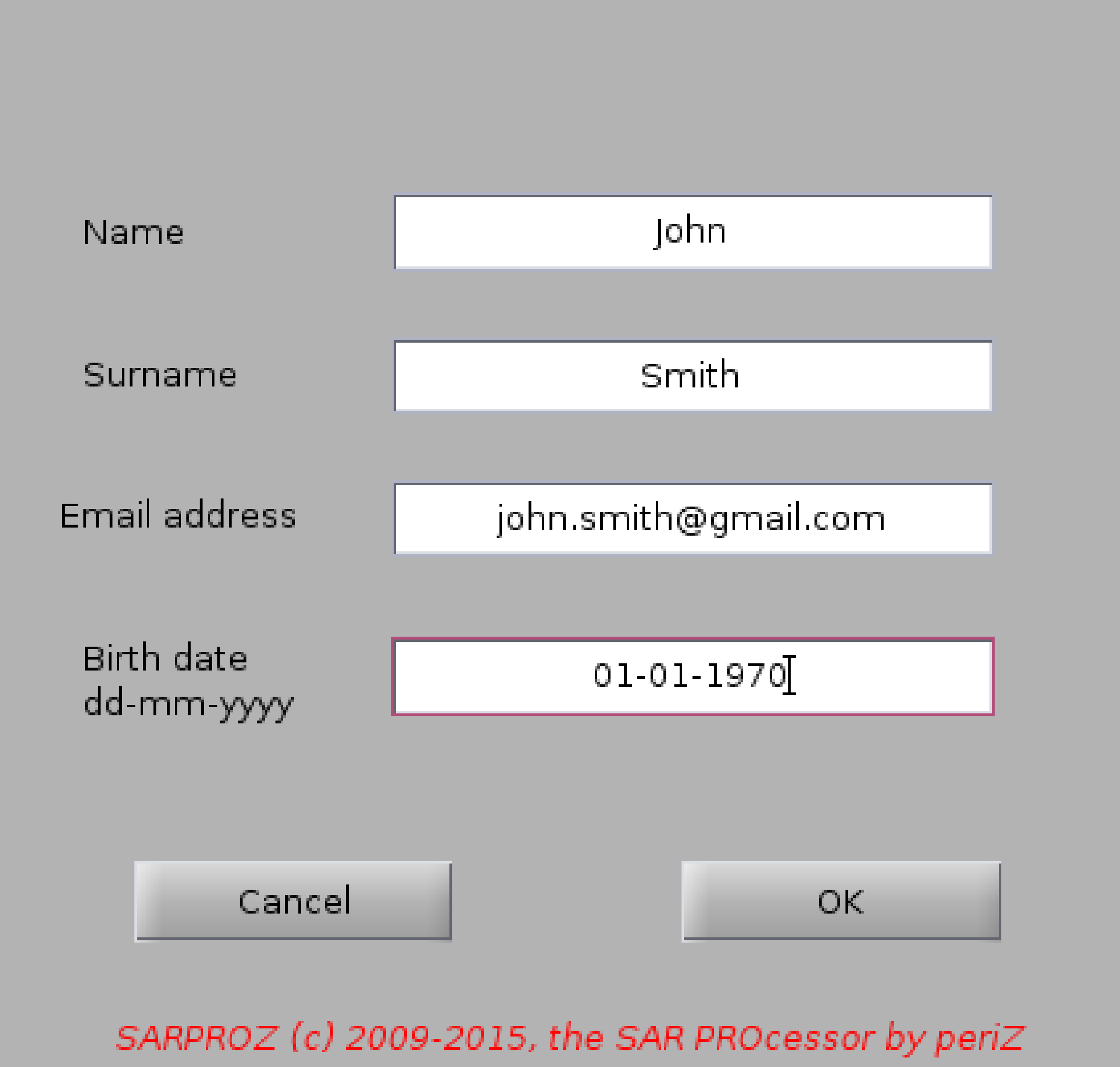
Help for Personal Data reporting for license generation
This window is opened at the first execution of SARPROZ.
Fill all fields with your personal information, an encrypted file will be generated to indentify
the user and its machine.
SARPROZ will attempt to automatically send the file by email asking for the authorized license file.
If the automatic sending fails, the user is asked to send the license file manually.
The authorized license file will be sent to the email address written in this form.
In case of installation on multiple machines, please modify your name to univocally identify the
machine on which you are installing the software (eg: PC1, PC2 and so on)
Please note that the license file MUST be created by running the software on the target machine.
You cannot run the software on a machine "A" asking for a license for a machine "B".
Please note that SARPROZ always gives messages about success/failure of operations.
If the license is correctly generated and sent by email, simply wait for an answer by email.
If something wrong happens, SARPROZ will tell you that.
If the license is NOT correctly generated, you cannot get authorization to run the software. So, you need to generate a new license.key file.
To generate a new license.key file you have to delete the old one and run the software again.
More information on the installation can be found in the Sarproz FAQ
http://www.sarproz.com/sarproz-faq/
or in the installation instructions
http://www.sarproz.com/installation-instructions/
Note that SARPROZ needs an internet connection to start.
Back to main index
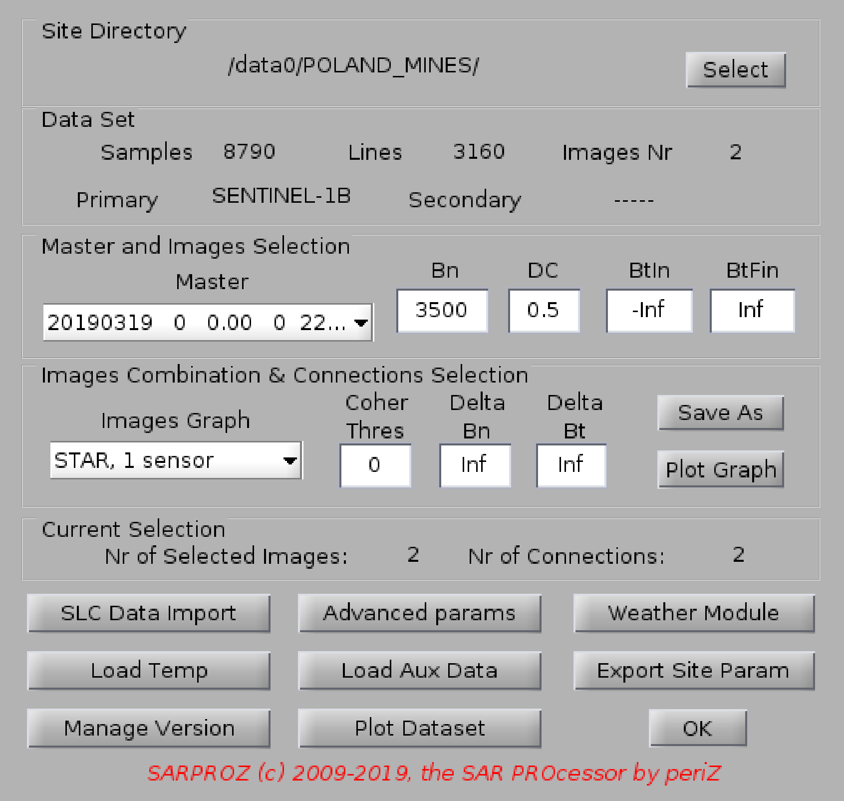
Help for DATASET SELECTION
With this function you can select the dataset to process
Press the Select button and choose a directory
es: c:\my_data\my_site is your DataSet directory
At this moment, Sarproz is not including a focusing module.
Thus, you can import in Sarproz the following formats:
a. SLC data (not-registered, as provided by data distributors or focused by other sw)
--> place data in folder SLC
b. co-registered SLC data
--> place data in folder RSLC
a. SLC data.
* Sensors currently supported as provided by data distributors:
- ERS 1-2 and Envisat
- Cosmo 1-2-3-4
- TerraSAR-X and Tandem-X
- ALOS (JAXA and ERSDAC)
- RadarSAT 1-2
- Sentinel 1
- Kompsat-5
Simply place the data in a directory called SLC within the DataSet directory (e.g. c:\my_data\my_site\SLC).
Sarproz will automatically detect the data format and sub-directories trees.
In Linux, data are un-tared or un-zipped automatically by the software.
In windows, you should create a directory for each image (and you may need to un-tar/un-zip data manually).
* data focused by other software:
- ROI_PAC: ERS-Envisat-ALOS (for adding other sensors, please contact the administrator. a few quick changes are needed)
Place yyyymmdd.slc and yyyymmdd.slc.rsc files in the folder SLC (do not use sub-directories).
! for ALOS ROI_PAC: Rename all LED-ALPSRP*********-H1.0__A files into yyyymmdd.led and place them in the SLC folder !
- GAMMA: at this moment this option is not implemented. However, it can be done quickly in case of need.
Contact the administrator for that.
b. co-registered SLC data
- Any sensor supported by Gamma can be imported
simply place all registered SLC files (.rslc) and the parameters files (.rslc.par)
in a directory called RSLC within the site directory (e.g. c:\my_data\my_site\RSLC)
file names must be in the form yyyymmdd
The software will operate automatically a conversion
- for importing data co-registered by ROI_PAC, please contact the administrator
Once data are imported in Sarproz, the site can be accessed at any time
simply selecting the directory that contains the generated directory tree
(es c:\my_data\my_site)
After loading the dataset, the size of the images will be shown in the window DATASET SELECTION
(Samples in Range and Lines in Azimuth)
The name of the used sensor (as ERS or Envisat, TerraSAR, ALOS, CosmoSky-med, RadarSAT, Kompsat)
will appear in the field Primary
The software has also the possibility of processing two sensors together (as ERS and Envisat. See References).
To do this, you need to create an other folder within the DataSet directory.
The folder must be named with the second used sensors (e.g. c:\my_data\my_site\ENVISAT if the second sensor is Envisat)
At the moment this option is implemented for: ENVISAT, ERS, RADARSAT
The second dataset must be independently converted into the software format
With this function you can also choose a different Master Image (choosing among the available images)
You can put thresholds on Normal Baseline and Doppler Centroid to reduce the set of images
to process
Moreover, the software gives you the possibility to choose which pairs of images to process for interferometric and multi-image purposes:
Through the menu "images graph" you can choose among:
-STAR graph, 1 sensor
-STAR graph, 2 sensors, 1 master (coherent combination)
-STAR graph, 2 sensors, 2 masters (un-coherent combination)
-MST (Minimum Spanning Tree, obtained by maximizing the coherence of all interferograms), 1 sensor
-MST, 2 sensors
-Full Graph (all possible connesctions)
-Small Temporal Baselines
You can download weather data from Internet using the button "Get Weather Data"
You can import your own temperature data using the button "Load Temp". Such values are used in the time series processing for estimating the thermal expansion.
The format must be a txt file with as many values as the images
in your dataset. Be careful: no check is carried out on the imported data. Temperature must be taken at the satellite acquisition time.
If you want to switch back to automatic temperature data downloaded by the software, press the button "Load Temp" and then cancel the operation.
You can also import other auxiliary data using the button "Load Aux Data". Such data will be used instead of Doppler Centroid values.
So that you may estimate a dependency of the phase values on your parameter (currently the subpixel azimuth position can be estimated using DC values).
Be careful (1): Doppler is here referred to the PRF.
Be careful (2): a threshold is applied by the software to Doppler values. It means you have to either normalize your data to the same
range of values or you have to modify the Doppler threshold.
If you want to switch back to real Doppler values, press the button "Load Aux Data" and then cancel the operation.
Finally, you can export the site parameters through the button "Export Site Param". Such function will generate a ExportPar.tgz file which can be sent to other people
for replicating your site parameters. You have to include such file together with other mat files you want to share (e.g. AutoConnex.mat if you want to share
your APS processing results with others, or any files in RESULTS/GUIDE if you want to send a small area)
References:
D. Perissin, C. Prati, M. Engdahl, Y.-L. Desnos, "Validating the SAR wave-number shift principle
with ERS-Envisat PS coherent combination", IEEE Transactions on Geoscience and Remote Sensing,
Volume 44, Issue 9, Sept. 2006 Pages: 2343 - 2351.
1.2.1. SLC Data Processing
1.2.2. Advanced Parameters
1.2.3. Manage Version
Back to main index
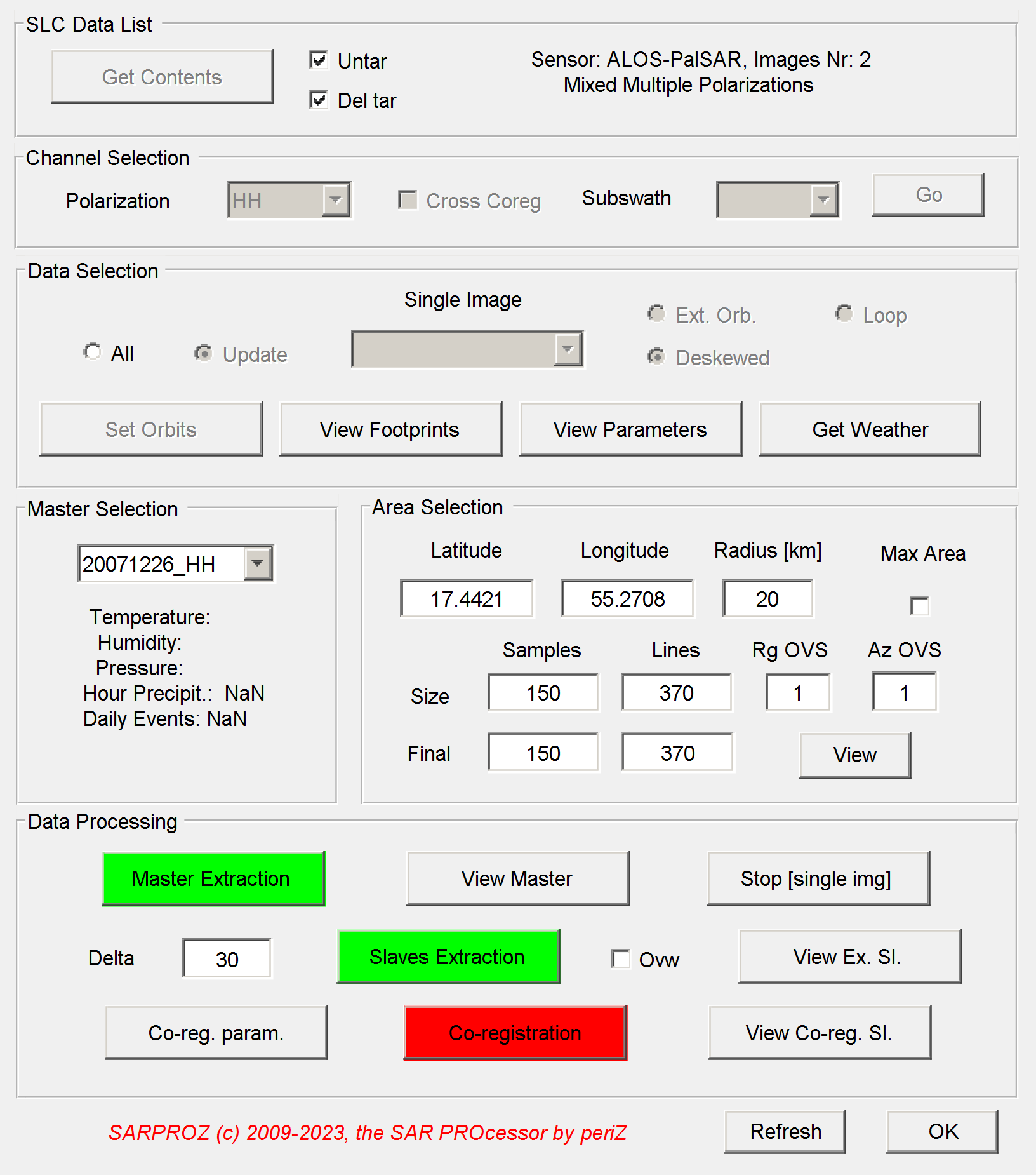
1.2.1. SLC Data Processing
SLC data module
Up
With this module you can import SLC data.
1) place your SLC data in the SLC folder in the dataset directory (e.g. c:\my_syte\SLC)
2) by selecting the directory "c:\my_site" from the dataset "selection module", if the directory SLC is found in "c:\my_site", the SLC module will be
automatically opened
3) press the button "Get Contents": the software will analyze the content of the SLC folder and give you a report.
some information is written on the window, in the SLC Data List frame, like Sensor, Number of Images, Polarizations
some information is also printed on the screen. The tool is checking also orbits, acquisition mode and so on: only interferometric datasets are
supported.
OPTIONS
-Untar: if this option is selected, tar, zip, gzip files are extracted. This option is not working under windows
-DelTar: if this option is selected, after a successfull extraction, the zipped files are removed
4) if options are given (e.g. you are importing a dataset with multiple polarizations) check the polarization you want to work with from the "Polarization"
frame.
5) For creating a new dataset, keep the option "All" in the "Data Selection" frame and press "Set Orbits". The tool will read the orbits from the SLC data.
OPTIONS
-If a dataset was previously created, you can import new images with the "Update" option. All new SLC data placed in the SLC folder will be imported
-You can also choose to import a single new image by selecting it from the "Single Image" menu.
-If a dataset was previously created and you want to remove all previous results and start over again, you can keep the "All" option
and press the "Set Orbits" button again. A security window will be opened to ask for a confirm.
-The option "Ext. Orb." allows importing external orbits. Currently, this option is implemented only for ERS and Envisat. When importing ERS and
Envisat, the option is automatically selected. [check the note at the bottom for more details about external orbits]
-Weather data can be optionally downloaded at this stage. This may be useful to check whether any precipitation occurred at the Master date.
6) After setting the orbits, the footprints can be visualized in Google Earth by pressing the "View Footprints" button. Google Earth should be automatically
opened. If this creates problems, it can be disabled from the "Advanced Parameters" in the "dataset selection" window.
7) Also an estimation of the dataset parameters can be visualized by pressing the "View Parameters" button.
8) After setting the orbits, an automatic Master image is proposed. By plotting the parameters and/or by downloading weather data, the Master may be
changed manually.
9) After selecting the Master, the area to be extracted can be set up from the "Area Selection" frame.
OPTIONS
-the center coordinates of the area to be extracted can be changed using the Latitude/Longitude text input boxes
-the area can be set up by inputing a radius [km] in the corresponding box
-the tick "Max Area" allows selecting the maximum common are of the dataset footprints
-the final image size can be manually set using the corresponding boxes
-also the oversampling factors in range and azimith can here be chosen
10) Once the area is set, it is poossible to visualize it in Google Earth pressing the button "View"
11) After Master and Area are given, data can be extracted starting from the Master image ("Master Extraction")
12) The Master image can then be plotted pressing the button "View Master"
OPTION
-if a single image is imported, the dataset can be closed using the button "Stop [single img]". This option can be used to extract and visualize
a single image.
13) Consequently, Slave images can be extracted with the button "Slave Extraction"
OPTIONS
-the slave image must be bigger than the Master one, to allow searching for the matching area. This is achived by giving a "Delta" in pixels.
Should the coregistration fail, Slave images can be visually checked. If a big shift w.r.t. the Master image is visible, the "Delta"
should be increased till assuring enough overlap with the Master image.
-if a slave images was already etracted and a wider image is needed with a higher Delta, the "Ovw" -overwrite- tick must be checked.
14) Extracted Slave images can be visualized with the button "View Ex. Sl."
15) Once Slave images are extracted, they can be coregistered using the button "Co-registration".
OPTIONS
Co-registration parameters can be changed using the "Co-reg. param" button.
See the Help for Co-registration Parameters.
16) To conclude, co-registered images can be displayed pressing the button "View co-reg. Sl."
[note for external orbits]
ERS and Envisat need external orbits.
The orbits are automatically downloaded from internet.
Should the process fail, external orbits are organized as follows:
- external orbits are saved in an ORBITS folder at the root of your data folder
e.g. c:\data\ers_dataset is your dataset folder
external orbits are stored in c:\data\ORBITS
- internal structure:
ORBITS\ENVISAT\yyyymm
ORBITS\ERS1\yyyy
ORBITS\ERS2\yyyy
- DOR_VOR orbits are used for Envisat
- PRC orbits for ERS
1.2.1.1. Coregistration Parameters
Back to main index
1.2.1.1. Coregistration Parameters
Up
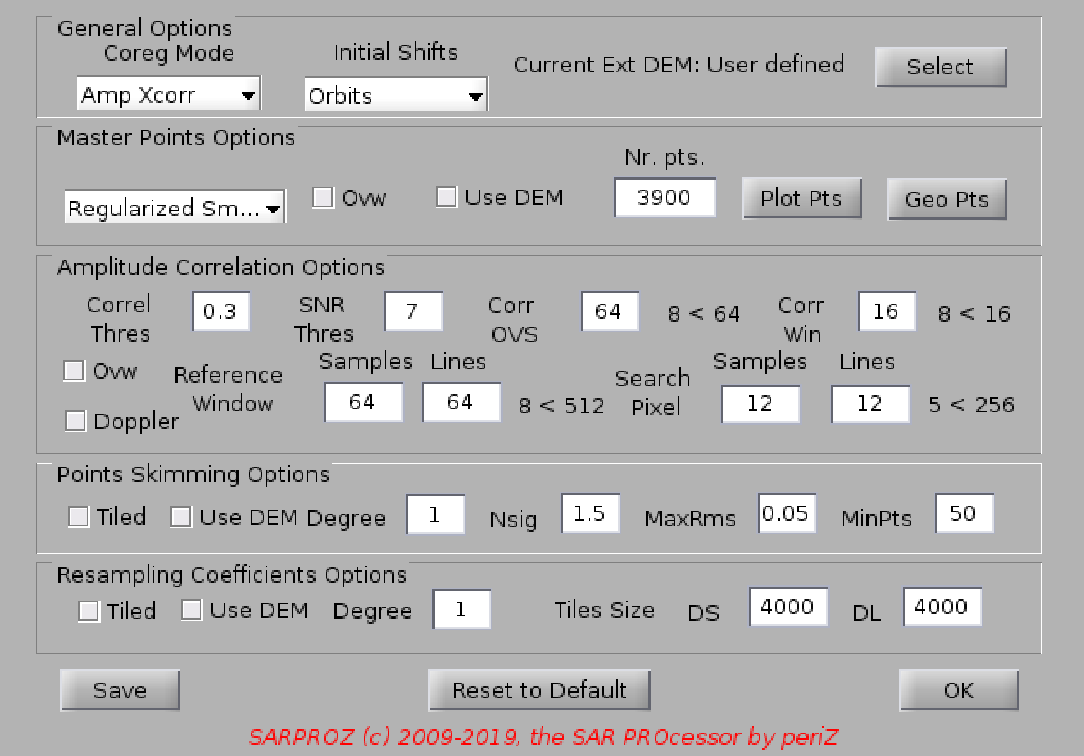
Help for Co-registration Parameters
Available Options:
1. Initial Shifts, from Orbits (default) or from Coarse Xcorr.
If the orbits are precise (like for new satellites) the initial shifts can be precisely determined. In such case, all default parameters
should work simply fine.
However, for satellites like Radarsat (but also to some extents ERS and Envisat), initial offsets may be wrong. In such cases, it is
better to use an initial coarse cross-correlation to estimate them instead of increasing the search pixels.
2. Smart option (default)
If selected, the fine cross-correlation is carried out on a set of point-like targets, extracted from the Master image.
Otherwise, the fine cross-correlation is carried out on a set of equally distributed points
3. Use Ext. DEM.
If selected, the height of the points used for the fine cross-correlation is extracted from the available external DEM (SRTM by default).
Otherwise, points are taken at a common height (usually at the scence center)
4. Nr of points.
Nr of initial points for fine cross-correlation. The number is automatically calculated by default.
5. Ovw Smart.
If selected, the initial set of points is overwritten. Otherwise, if a previous file is available, it is used by default.
6. Auto correction.
If selected, after a coregistration failure it tries to change a series of options to achieve success.
At this moment, if a failure occurs and if the initial shifts were calculated using orbital information, it tries to re-estimate then
via coarse cross-correlation. More options are under development.
7. Correlation threshold and SNR threshold
Used for selecting good cross-correlation matches.
8. Reference window
Size in Samples and Lines of the reference window. It can be increased in case of uncorrelated areas to improve the SNR.
The button "+" automatically increases the values, also based on the oversampling factors.
9. Search Pixel
Range of the searched shifts in the cross-correlation. It can be increased automatically by pressing the button "+".
10. Nsig, MaxRms, MiPts
Used for the final selection of the best good cross-correlation results.
11. Save
If parameters are changed, to keep the changes the "Save" button must be pressed.
12. Reset to Default
To neglect changes and use default options, press the button "Reset". Afterward, save the selection.
Back to main index
1.2.2. Advanced Parameters
Up
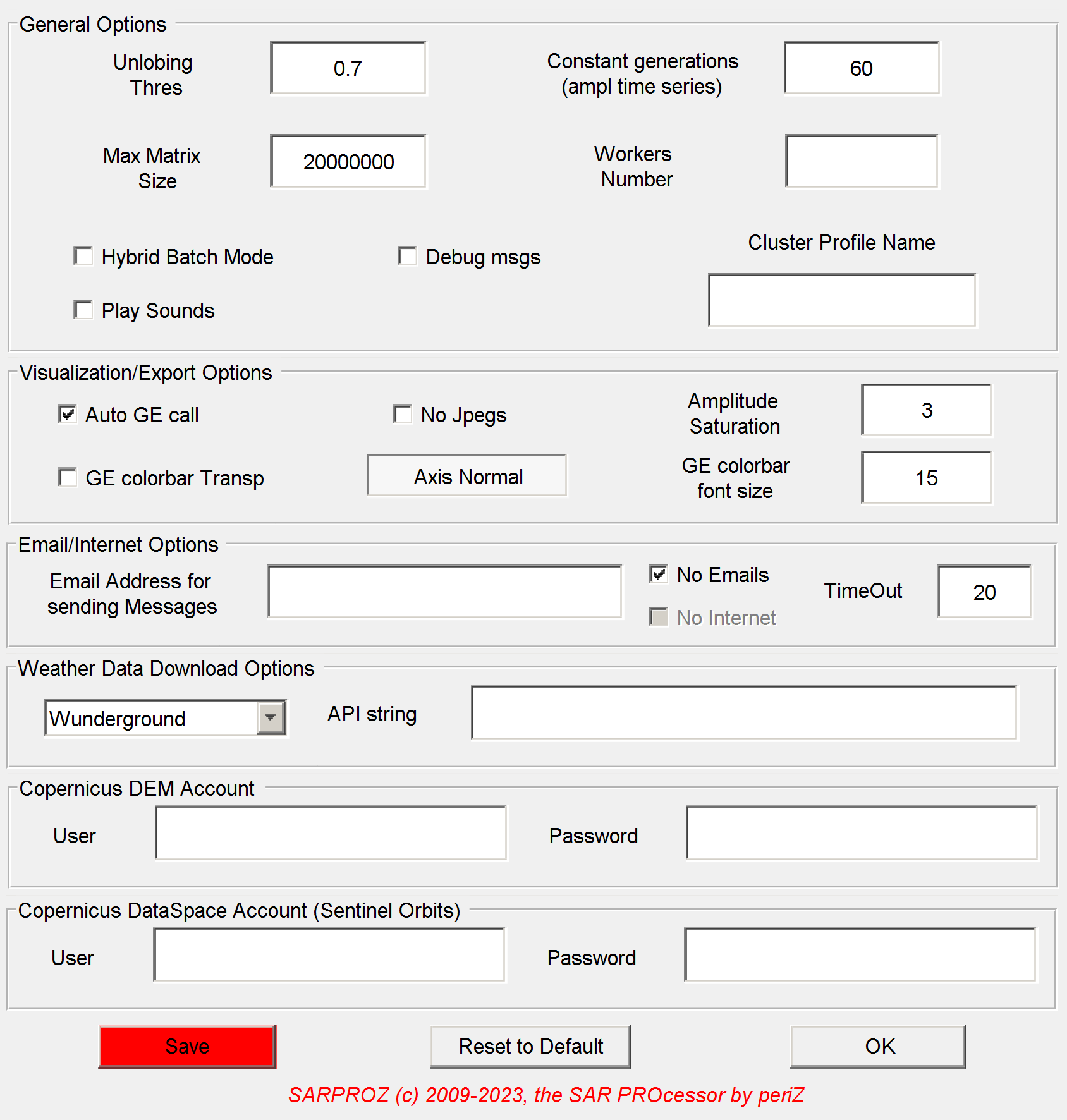
Help for advanced parameters
With this window you can modify some default parameters.
NOTE: you should not need to modify anything in normal conditions.
In case you get Out of Memory problems, you can try to decrease the "Maximum Matrix Size" value.
The "Amplitude Saturation" is the upper limit of amplitude values plotted in the corresponding images in the tool.
Eg for plotting a brighter image of the Reflectivity Map, decrease the value of "Amplitude Saturation".
Constant generation is a parameter for the genetic algorithms implementation of the Amplitude Time Series Analysis.
Unlobing threshold refers to the side lobes suppression in the Mask creation.
CPU Number is the number of parallel CPUs to be used.
Axis Image / Axis Normal. By default Sarproz plots anything in SAR coordinates keeping a ratio 1:1
between samples and lines (Axis Image). If you want a free ratio, switch to Axis Normal.
Back to main index
1.2.3. Manage Version
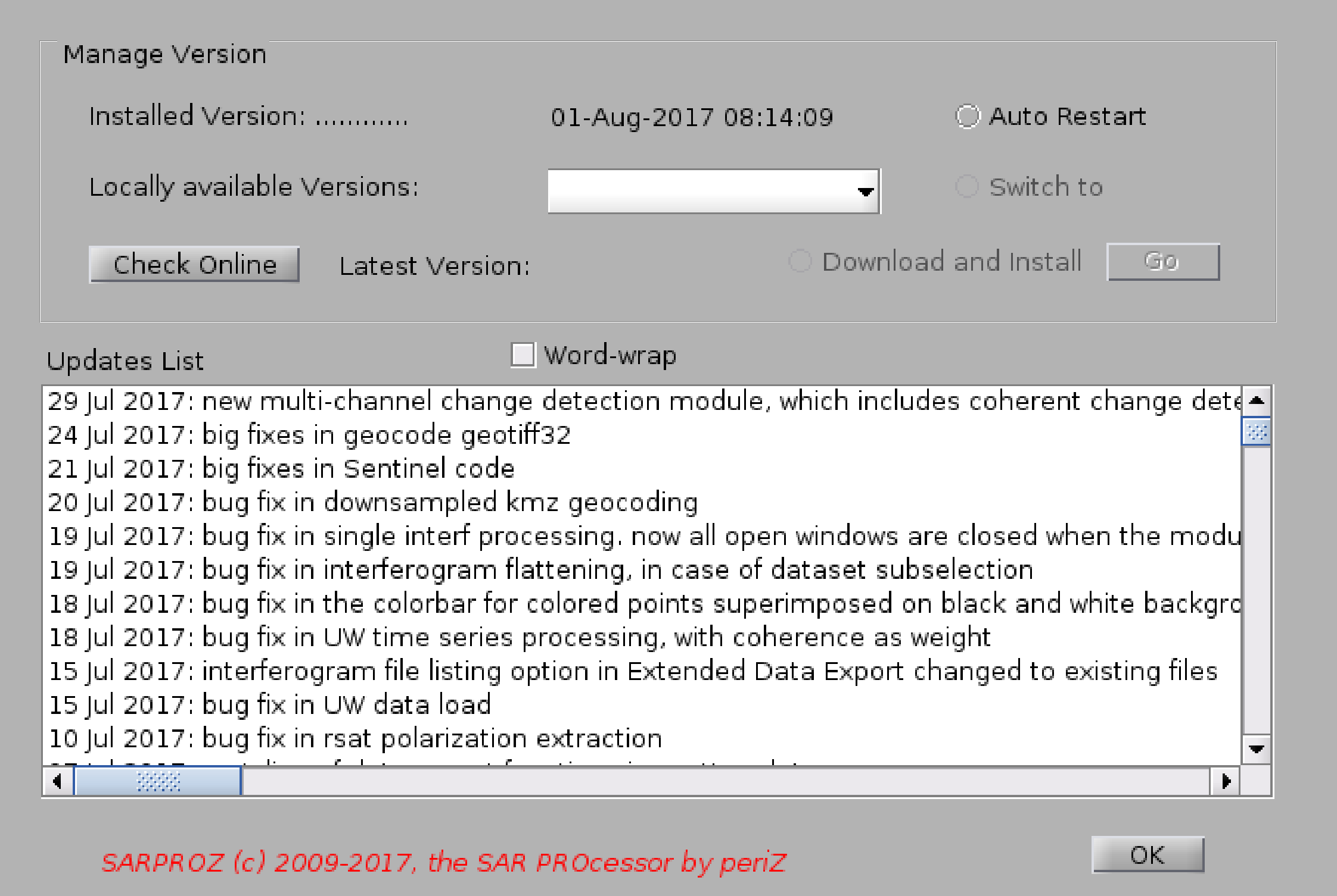
Help for Manage Version
Up
This module allows the following operations:
- check and download new software releases
- displaying the list of software updates in chronological order
- displaying the available local software versions (backups of old versions)
- switching between different software versions
This module is particularly useful for downloading the last available Sarproz version.
Moreover, since in some particular cases a new update may bring unstable behavior in untested circumstances,
the software gives the possibility to switch back to a previous release to overcome possible unstable situations.
A backup copy of each software version is automatically saved in a folder named "archive" inside the pcodes/compiled directory.
Naming convention is pcodes/compiled/compiled_linux_yyyy-mm-dd.tar
This module is compatible with older software versions (be reminded of the license change happened in Nov 2014).
To access this module in Sarproz versions where the button "Manage Version" in "DataSet Selection" was not present (for the pcodes release),
launch the command "manage_version(fig)" at the Matlab command prompt (for that, you must have already installed a software version later than 22 Feb 2015).
If you are running a compiled version, you cannot access this module in releases older than Feb 22nd 2015.
Back to main index
help for DATASET STATISTICS
this function plots the basic parameters of the dataset:
-histogram of normal baselines
-histogram of Doppler Centroid values
-temporal series of the acquistions, denoting which ones are used in the
PS analysis, according to the thresholds written in the Select DataSet
window. Colors are used to distinguish between sensors. The Master image is
highlighted as well.
-time series of the temperatures at the acquisition time
Back to main index
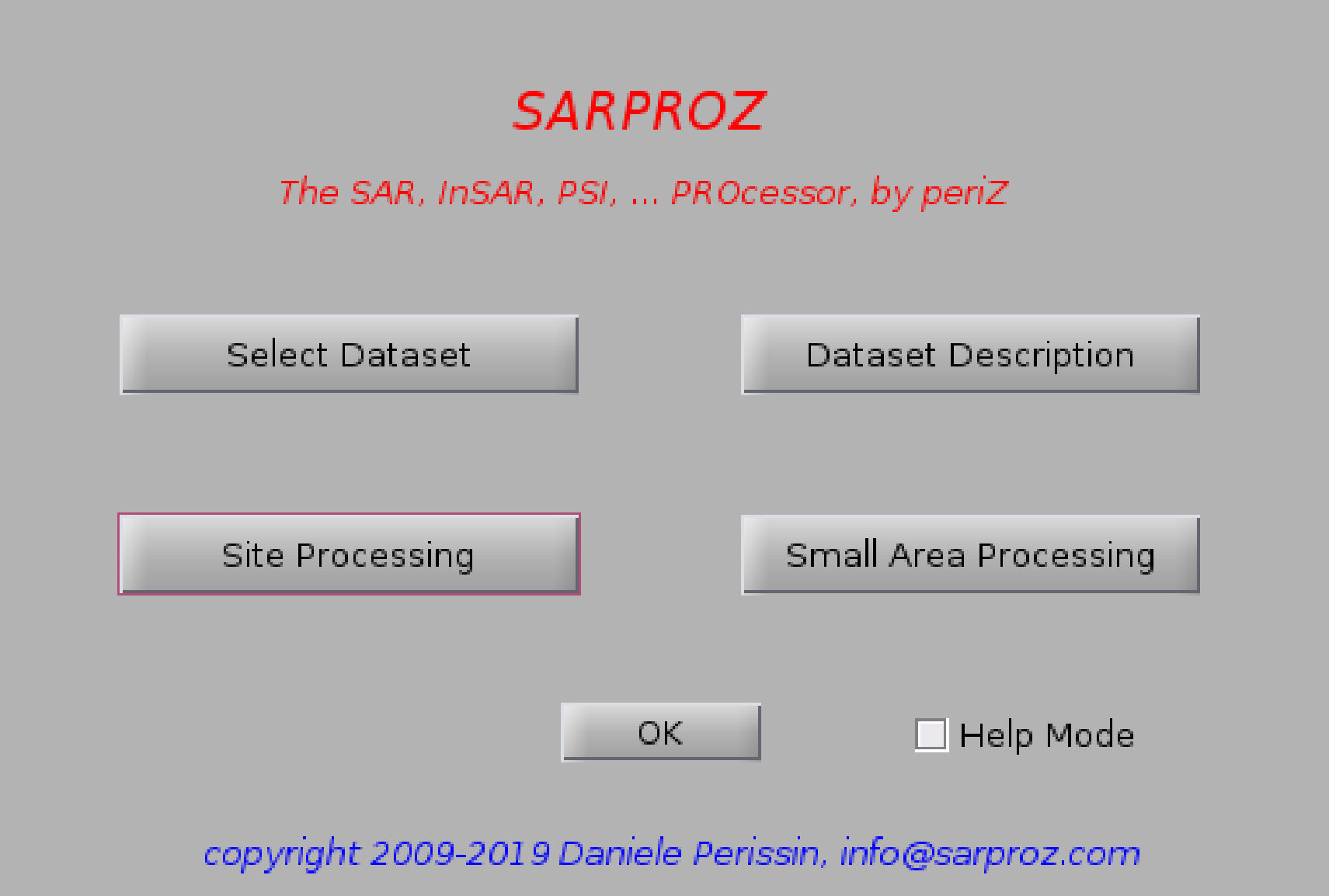
Help for Site Processing
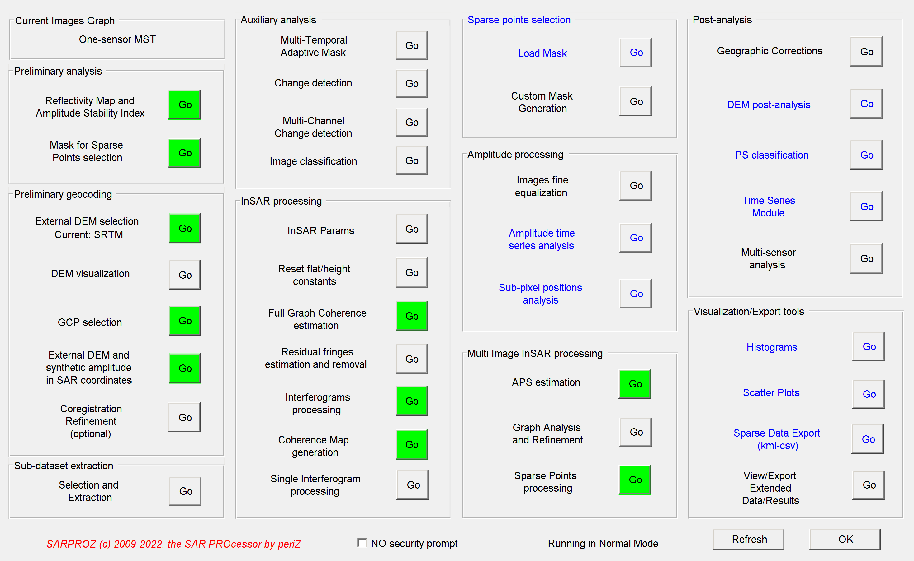
Within this window you can choose among many operations to perform on your dataset.
The functions are divided into 10 groups:
-Preliminary analysis (to be performed as first)
-Preliminary geocoding (to correct initial orbit offsets)
-Amplitude processing (to process amplitude time series)
-InSAR processing (to prepare and perform interferometric analysis)
-Multi Image InSAR processing (to implement PS-QPS approaches)
-Visualization tools (to view data and results)
-Sparse points selection (to select sparse points on which running the functions written in blue)
-Post-analysis (to be performed after multi-mage InSAR processing)
-Auxiliary analysis (as change detection and image classification)
-Results reporting (to export results)
Some functions are written in blue: those functions apply to sparse points analysis instead of processing all image pixels.
Some functions can be performed without specifying any other options or without opening other dialog windows: to avoid starting
long processing operations by mistake, the user is asked for a confirmation through a window that appears for 5 seconds.
If no confirmation is given, the command is aborted. To avoid such security prompt, you can check the corresponding option
on the site processing window.
Site processing functions are not included in the Demo version.
1.4.1. Preliminary Analysis
1.4.2. Preliminary Geocoding
1.4.3. InSAR Processing
1.4.4. Sparse Points Selection
1.4.5. Amplitude Processing
1.4.6. Multi-Image InSAR Processing
1.4.7. Post Analysis
1.4.8. Auxiliary Analysis
1.4.9. Visualization Tools
1.4.10. Results Exporting
1.4.11. Sub-dataset Extraction
Back to main index
1.4.1. Preliminary Analysis Up
1.4.1.1. Reflectivity Map
1.4.1.2. Mask Generation
1.4.1.3. Sar2geo Coefficients
Back to main index
1.4.1.1. Reflectivity Map Up
Help for Reflectivity Map and Amplitude Stability Index
With this function the tool generates the Reflectivity Map as the temporal average
of all images of the dataset that have been chosen to process
(see DataSet Selection)
The tool processes also the Temporal Standard Deviation and saves the
MuSuSigma (mean devided by std) matrix.
Files are saved in the directory RESULTS in the DataSet directory.
In case of 2 sensors analysis, two different Refl Maps are processed and saved
They are called respectively MeanFirst and MeanSecond
The final results can be diplayed with the function "View Parameters".
Back to main index
1.4.1.2. Mask Generation
Up
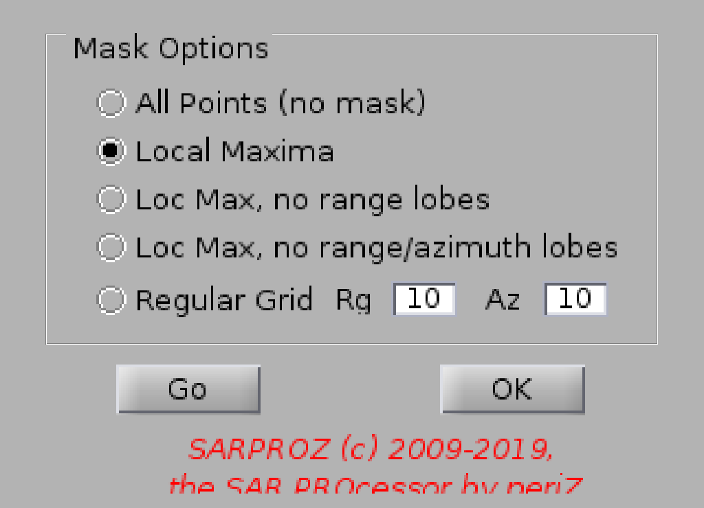
Help for Mask creation
This function creates a mask for sparse points selection.
The mask is used by all functions that implement sparse points analysis
that is, PS (QPS) processing and all functions written in blue in the Site Processing window
In general, the mask is used everytime a selection of points is applied.
The function allows to choose among (see references):
-all points (no mask)
-local maxima extraction (from the Reflectivity Map)
-local maxima extraction with range lobes suppression
-local maxima extraction with range and azimuth lobes suppression
-regular grid, spaced dS by dL
The function creates a matlab sparse matrix in the directory RESULTS called Maschera.mat.
If the file Maschera.mat does not exist, all points are selected.
If NO security prompt is selected, no windows is opened, local maxima are selected by default.
If NO security prompt is NOT selected, the tool open a winows for choosing the option.
See the Small Area Processing for a detailed analysis on a sub-region (Amplitude Analysis).
References:
D. Perissin, F. Rocca, "High accuracy urban DEM using Permanent Scatterers",
IEEE Transactions on Geoscience and Remote Sensing, Volume 44, Issue 11, Nov. 2006 Pages: 3338 - 3347.
Back to main index
1.4.1.3. Sar2geo Coefficients Help for sar2geo / geo2sar coeffs
Up
This processing step is not strictly required.
Running this function will save time during any geo2sar/sar2geo processing operation.
However, it takes itself some time to be exectuted and it represents an approximation (erros are anyway negligible).
Useful for big sites. Unnecessary for small sites.
For new generation satellites, for which orbits are quite precise and straight, running this
function will take little time and speed up further operations.
For old satellites as ERS and Envisat, this operation will take some time more.
We leave the choice to the user.
Back to main index
1.4.2. Preliminary Geocoding Up
1.4.2.1. External DEM Selection
1.4.2.2. DEM Visualization
1.4.2.3. Geocoding through GCP
1.4.2.4. Ext. DEM in SAR Coordinates
Back to main index
1.4.2.1. External DEM Selection
Up
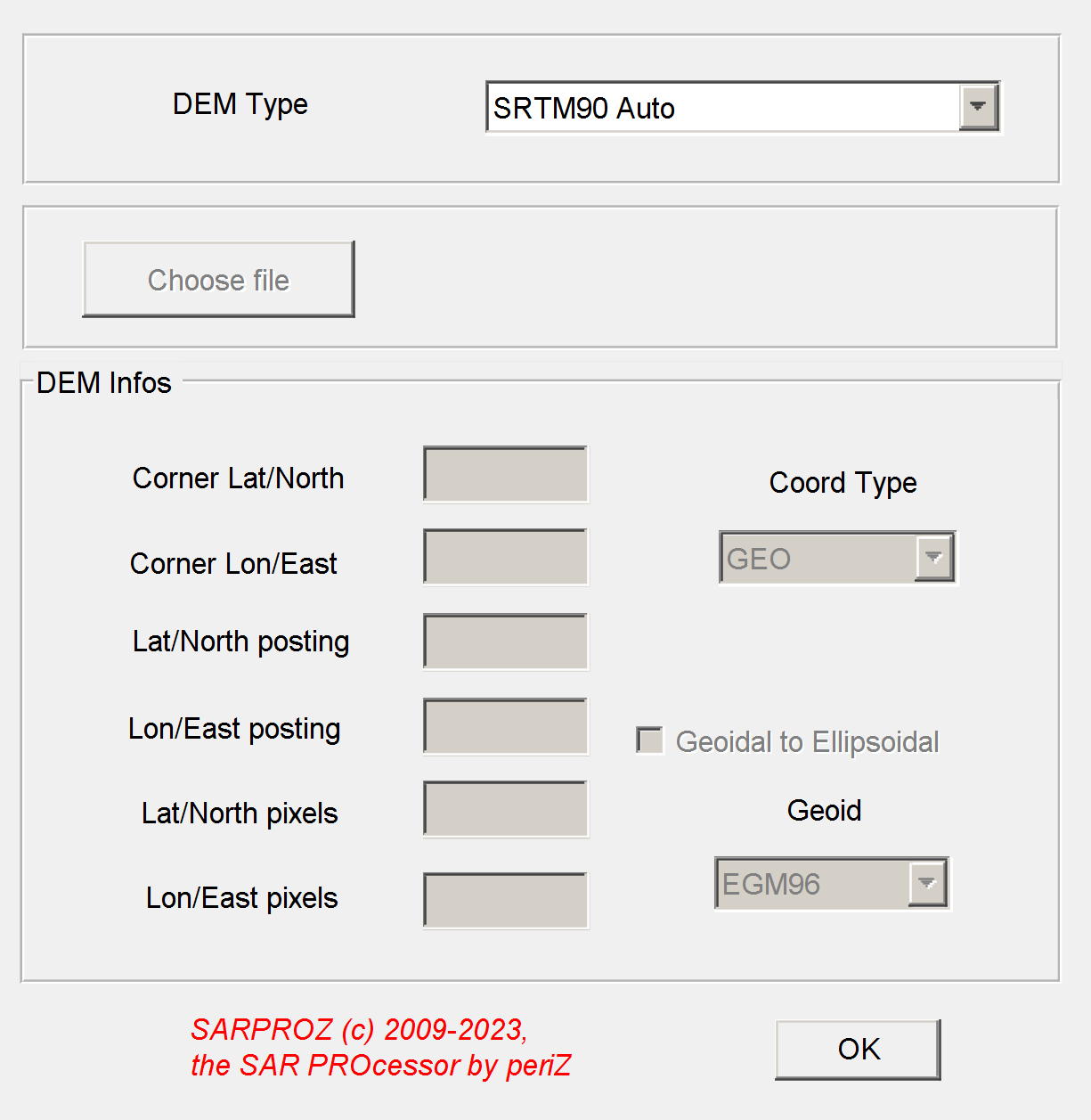
Help for External DEM Selection
With this function you can choose the source of your External DEM
The default external DEM is SRTM (see notes)
To manually choose SRTM, press the button "Reset"
Otherwise, have 2 options:
a) loading a GEOTIFF file. Do this via "Choose file" and select the corresponding tif file
If the file is correctly identified and read, all parameters are automatically filled.
b) loading a matrix, described by the parameters visible in the window. Currently, the matrix must
be organized as a DEM file produced by Gamma. If a Gamma parameter file is available, it can be
imported via the button "Import par", and all parameters are automatically loaded
In the Gamma format, the matrix is organized as follows:
columns are Latitudes, rows are Longitudes, the file is float, big endian
Conversion between Geoidal and Ellipsoidal Height: work in progress
Notes:
The tool automatically downloads SRTM files from internet
If anything fails, a message is printed but the tool
does not stop running
SRTM files can be manually placed in DirSite/../SRTM
Back to main index
1.4.2.2. DEM Visualization Up
Help file for VIEW DEM
This function plots a matrix of height values
in Geographical coordinates
read from the choosen external DEM (SRTM by default)
Four black crosses are plotted in correspondence
of the SAR footprint of the DataSet
Notes:
When the tool reads SRTM, it prints on the screen
the files that are going to be read
If files are missing, a message is printed but the tool
does not stop running
SRTM files must be placed in DirSite/../SRTM
To choose an other external DEM, press the button
"External DEM selection"
Back to main index
1.4.2.3. Geocoding through GCP
Up
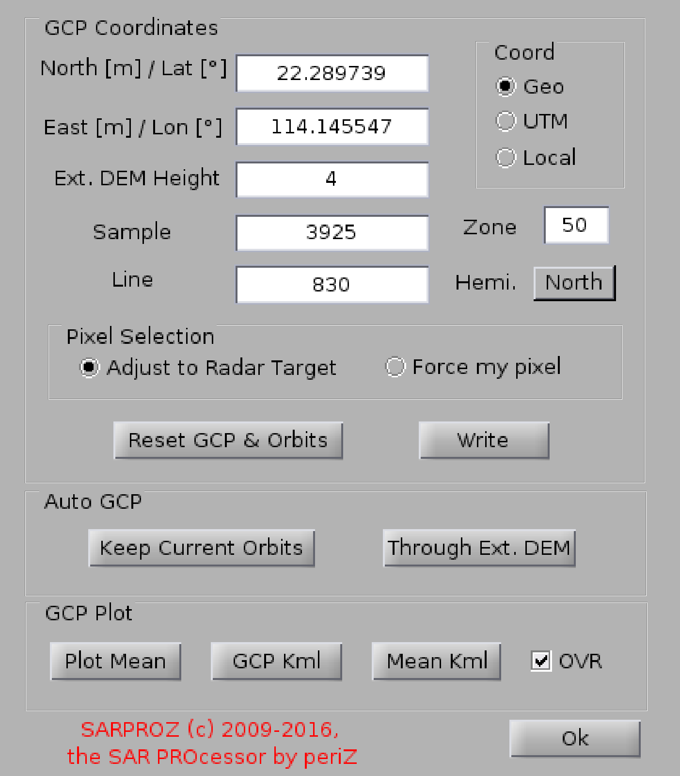
Help for Geocoding through GCP Selection
With this function the tool geocodes the DataSet through a Ground Control Point.
There are 3 options for inserting a GCP:
-manual
-automatic, through the external DEM
-automatic, without changing the current orbital offsets
Manual input:
Insert the GCP coordinates (Geographical or UTM -as for local coordinate systems,
at this moment only the Italian one is implemented-) and its position in the SAR grid
(Sample and Line). The Height is automatically extracted from the Ext. DEM.
After manual inputing, press the button "Write".
In case of errors, the GCP can be resetted and the original orbits are restored.
The GCP can be visualized on the Reflectivity Map (by pressing the button Plot Mean)
or in GoogleEarth (by pressing the kml button).
Also the Reflectivity map can be visualized in GE (downsampling 8 by 8).
The geocoded Refl. Map is read from the disk, unless the option "OVR" (overwrite) is selected.
After changing a GCP, to create a new geocoded Refl. Map and see the changes check the option "OVR".
Reference
D. Perissin, "Validation of the sub-metric accuracy of vertical positioning of PS's in C band",
IEEE Geoscience and Remote Sensing letters, Vol. 5, No. 3, July 2008, Pages: 502 - 506.
Back to main index
1.4.2.4. Ext. DEM in SAR Coordinates Up
Help for External DEM and Synthetic Amplitude in SAR coordinates
With this function the tool processes and writes the External DEM and Synthetic Amplitude in SAR coordinates.
The files are written in the RESULTS directory.
The final results can be diplayed with the fucntion "View Parameters".
Back to main index
1.4.3. InSAR Processing Up
1.4.3.1. InSAR Parameters Selection
1.4.3.2. Phase-to-height Constants
1.4.3.3. Phase-to-flat Constants
1.4.3.4. MST Estimation
1.4.3.5. Residual Fringes Removal
1.4.3.6. Second Order Fringes Removal
1.4.3.7. Interferograms Processing
1.4.3.8. Coherence Map Generation
1.4.3.9. Synthetic Coherence Map
1.4.3.10. Single Interferogram Processing
Back to main index
1.4.3.1. InSAR Parameters Selection
Help for InSAR Paramaters
Up
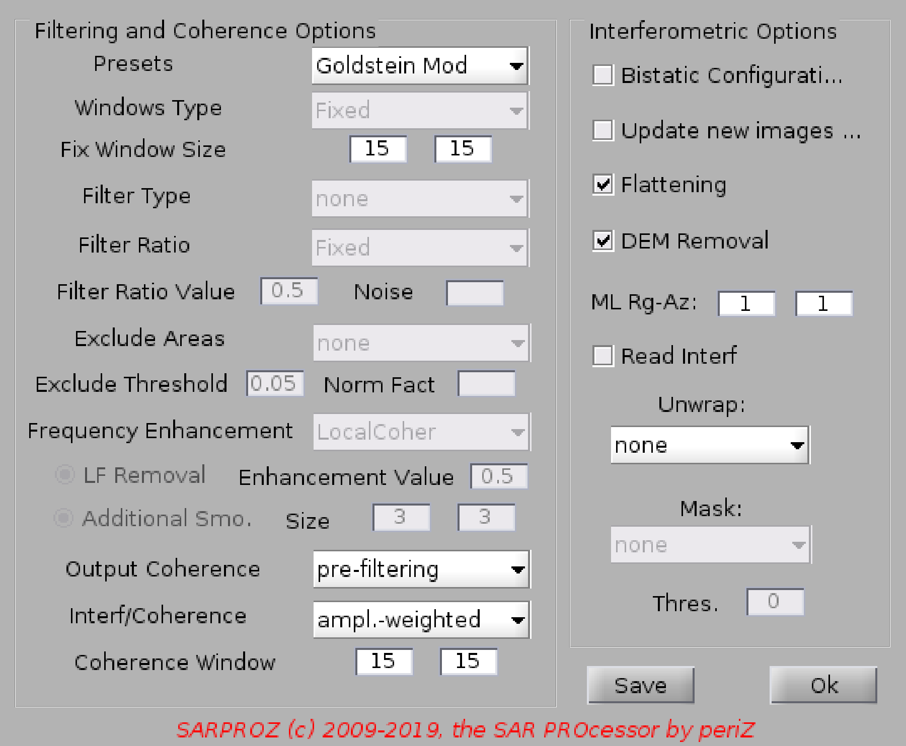
In this module you can choose the parameters for InSAR processing.
Be careful: the parameters are saved on the disk and they are loaded by the software in all next modules everytime interferograms are needed.
For instance, if you select multi-looking factors 10x10, if you try to plot the coherence map, the software will search for a 10x10 multilooked
coherence map.
Multilooked interferograms are saved on the disk with a name which includes the multilooking factors. In this way, the software distinguishes
interferograms with different multilooking factors.
However, the software makes no distinction between flattened/unflattened/DEM corrected interferograms: they are called with the same names.
So, be careful and be consistent in your choices.
Available options:
-Update option: allows processing only the new/missing images
-Bistatic configuration: useful for TanDEM-X bistatic pairs (automatically set)
This option modifies phase2flat and phase2height constants generation. If you change it, re-generate phase2flat and
phase2height constants
-Flattening: removes the flat terrain phase fringes
-DEM Removal: removes the topographic phase component (DEM in SAR coordinates must be available)
-Filtering: none/boxcar/Goldstein/MT adapt. Here you can choose which algorithm to use for filtering.
Window: filtering window size (samples by lines)
-Unwrap: unwrap fringes (WARNING: the full interferogram must be loaded: if the area is big, you need enough RAM)
-Conversion: converts the phase either in height [m] or in displacement [mm]
-Read & Unwrap: this is useful in case you previously processed an interferogram and now you want to unwrap it without
processing it again.
IMPORTANT NOTE:
Each interferogram is called with the following name: SLAVE_MASTER (see Interferogram Processing for more details on this).
The name does not change if you choose different processing options.
An unwrapped interferogram is called as SLAVE_MASTER_UW, regardless whether values are radians, meters or millimeters.
Be consistent with your operations!!!!!
Back to main index
1.4.3.2. Phase-to-height Constants Up
Help for Phase to Height Constants Generation
This function calculates Phase to Height Constants for removing the topographic phase term from
Interferograms or sparse points.
Back to main index
1.4.3.3. Phase-to-flat Constants Up
Help for Phase to Flat Constants Generation
This function calculates Phase to Flat Constants for Interferogram
(or sparse points) flattening (removal of flat terrain interferometric phase)
Back to main index
1.4.3.4. MST Estimation Up
Help for MST estimation
This function estimates the Minimum Spanning Tree of the images graph of the dataset.
In other words, the minimum best set of interferograms (graph links) connecting all available images
is generated by maximizing the coherence.
The MST is used for the QPS technique and for refining orbits (estimating residual fringes).
The tool handles both single and double sensor analysis, saving two different MST files.
After processing the MST, MST is automatically loaded as current Images Graph.
Thus, next processing steps can be executed using MST as current Images Graph.
References:
D. Perissin and T. Wang, "Repeat-pass SAR Interferometry with Partially Coherent Targets", submitted to TGARS.
D. Perissin, R. Piantanida, D. Piccagli, F. Rocca, "Landslide in Dossena (BG): comparison between
interferometric techniques", Proceedings of BIOGEOSAR 25-28 September 2007
Back to main index
1.4.3.5. Residual Fringes Removal Up
Help for Residual Fringes Estimation and Removal
This function estimates residual fringes from differential interferograms and refines
orbital data to better flatten interferograms.
WARNING: this function has been implemented for tackling some extreme cases of very poor
information about orbital data or related problems.
However, if the available orbital data are not particularly bad, it is not suggested to run
this function.
In fact, small residual orbital error can be estimated and removed also through APS estimation.
Moreover, in some cases long wavelength signals can be due to terrain motion.
While the APS estimation is carried out after estimating phase trends in time, at this step
fringes are removed from single interferograms without considering their correlation in time.
It is therefore recommended to run this function only when fringes are seriously affecting
further analysis.
In any case, it has to be kept in mind that all long wavelengths are canceled out,
and thus also possible terrain motion.
Back to main index
1.4.3.6. Second Order Fringes Removal
Up
Help for Second Order Fringes Removal
With this function you can correct possible second order fringes due to orbital inaccuracies.
This function is useless if you are processing a small area, it could become foundamental if you are processing
several frames together.
Back to main index
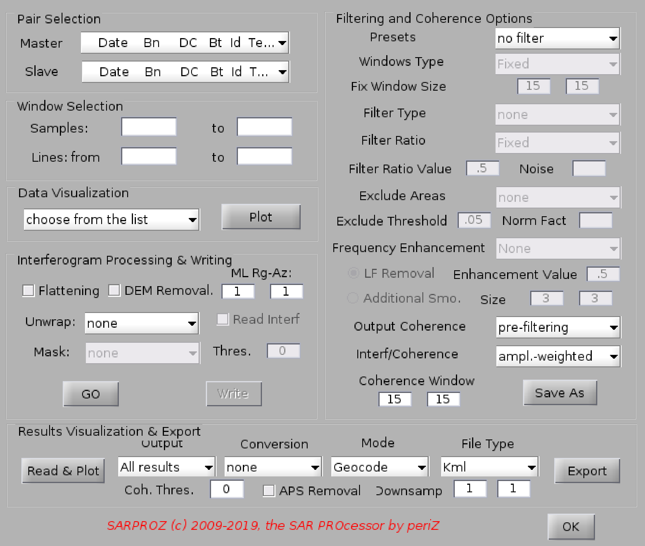
1.4.3.7. Interferograms Processing Up
Help for Interferogram Processing
With this function the tool processes interferograms according to the loaded images graph.
The options for interferogram processing can be chosen from the "InSAR Parameters" module.
Interferograms are saved as complex images, in which the phase is the interferometric phase and
the amplitude is the estimated coherence.
!!!!!!!!!!!!!!!!!!!!!!!!!!!!!!!!!!!!!!!!!!!!!!!!!!!!!!!!!!!!!!!!!!!!!!!!!!!!!!!!!!!!!!!!!!!!!!!!
SIGN OF INTERFEROGRAMS
There are 2 conventions for the interferograms sign, InSAR and PSInSAR.
InSAR: MASTER-SLAVE, and interferograms are written on disk with name SLAVE_MASTER.
However, PSInSAR uses the convention SLAVE-MASTER.
Thus, each line in the Images Incidence Matrix contains first a "1" and then a "-1",
corresponding to SLAVE (1) and MASTER (-1)
or likewise each line of the Graph Matrix contains indexes to SLAVE and MASTER images
(SLAVE,MASTER)
However, the corresponding interferogram saved in the directory "INTERFEROGRAMS", will
be named "SLAVE_MASTER" BUT it will contain the interferogram with opposite sign: MASTER-SLAVE
Back to main index
1.4.3.8. Coherence Map Generation Up
Help for Coherence Map Generation
This function reads the interferograms according to loaded Images Graph
and calculates the Spatial Coherence map as the average coherence of the set of current interferograms
The result can be plotted through View Parameters by choosing "Spatial Coher."
Back to main index
1.4.3.9. Synthetic Coherence Map Up
Help for Synhetic Coherence Map Generation
This function calculates the effective normal and temporal baseline dispersions for all pixels
and based on them a synthetic temporal coherence.
See References for further details.
The tool uses the images graph currently loaded and reads the corresponding interferograms previously created.
References:
D. Perissin and T. Wang, "Repeat-pass SAR Interferometry with Partially Coherent Targets", submitted to TGARS.
D. Perissin, R. Piantanida, D. Piccagli, F. Rocca, "Landslide in Dossena (BG): comparison between
interferometric techniques", Proceedings of BIOGEOSAR 25-28 September 2007
Back to main index
1.4.3.10. Single Interferogram Processing
Up
Help for Single Interferogram Processing
With this function you can choose freely one interferogram to process and visualize.
You can also process a smaller area and choose which operations to perform.
Back to main index
1.4.4. Sparse Points Selection Up
1.4.4.1. Load Mask
Back to main index
1.4.4.1. Load Mask
Up
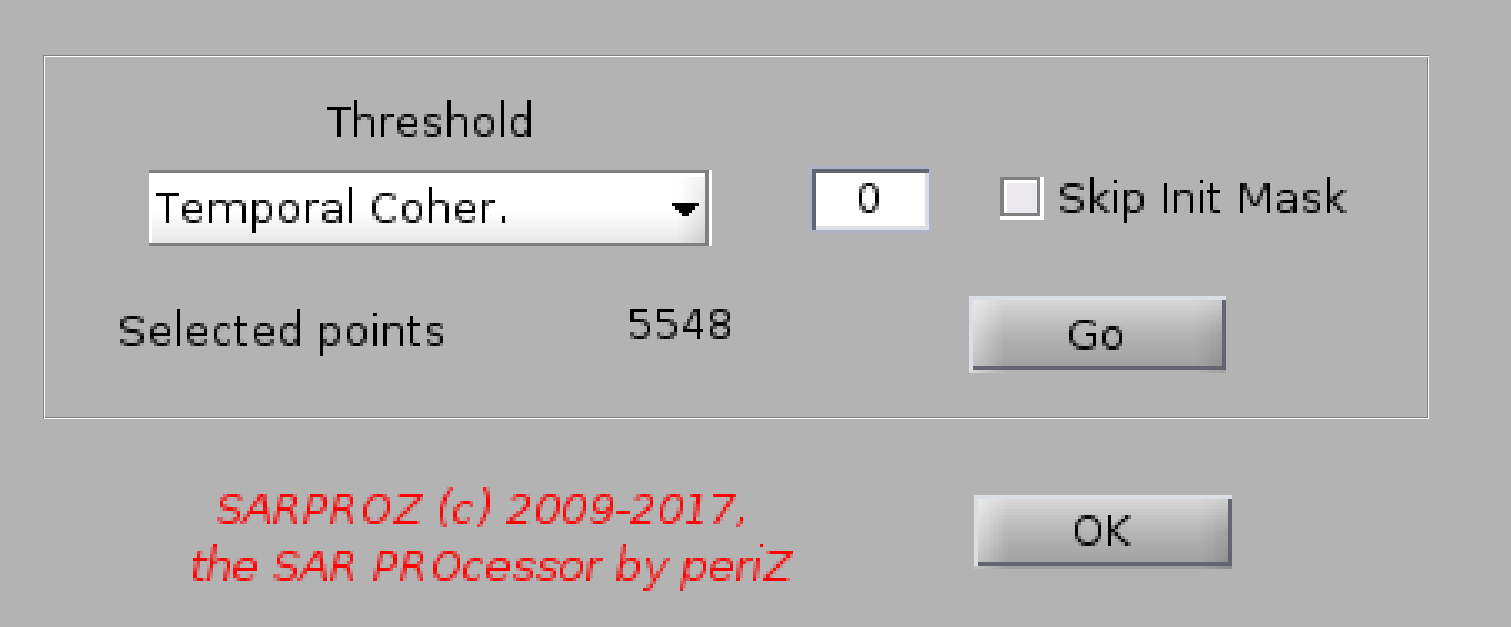
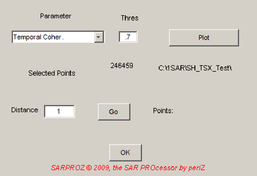
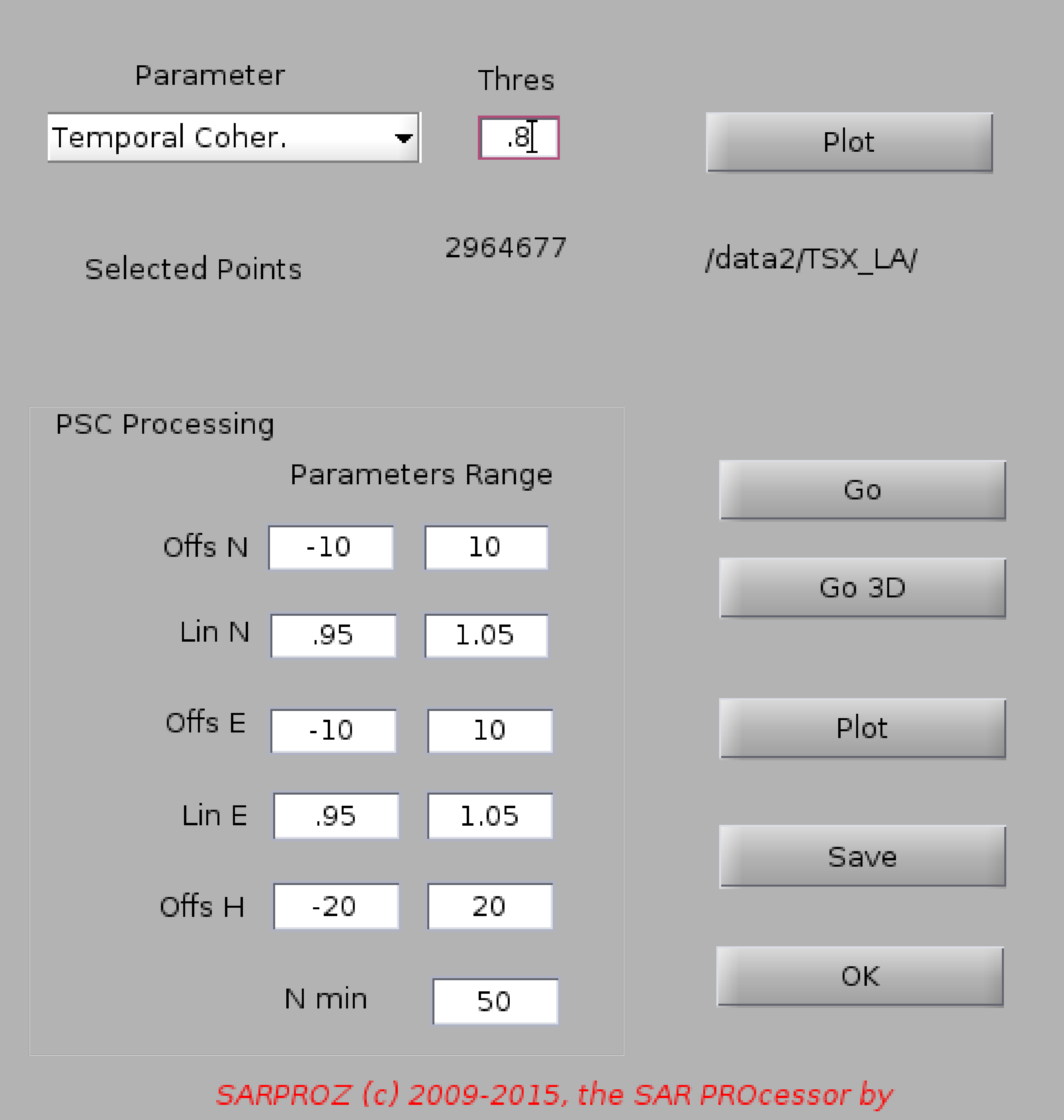
Help for Load mask
With this function you can select a set of sparse points on which performing sparse points analysis (functions written in blue
in the Site Processing window).
To select points, choose a parameter and specify a threshold. All points with paramter greater than the threshols will be extracted
and loaded in the workspace. If you want to perform more complex selections, read the following and use "Scatter Plots".
Note that if a MASK file has been generated, the points selection is restricted to the set of sparse points saved in the MASK file
(this is useful eg if you are interested in selecting point-wise targets and in discarding side lobes).
If on the contrary you want to select a set of points NOT restricted to the previosly created MASK file, rename or move the MASK file.
Here the set of parameters you can choose (note that you can also choose a new file created by yourself (line 47), e.g. with "Scatter Plots")
1
2 'Temporal Coherence'
3 'Res. Height [m]'
4 'Velocity [mm/year]'
5 'Phase Shift [rad]'
6 'Azimuth Position (phases) [m]'
7 'RCS [m^2]'
8 'Range Width [m]'
9 'Range Pointing (Bn) [m]'
10 'Azimuth Width [m]'
11 'Azimuth Pointing (DC) [Hz/PRF]'
12 'Birth Date [years]'
13 'Death Date [years]'
14 'Fitting Index'
15 'Slant Range Position Standard Deviation [pix]'
16 'AP ampl. rel.'
17 'AP VV-HH Phase [rad]'
18 'Samples [pix]'
19 'Lines [pix]'
20 'Phase to Temperature Proportionality [rad/degC]'
21 'Amplitude incoherent Mean'
22 'Slant Range Position in Amplitude Mean [pix]'
23 'Slant Range Position in Master Image [pix]'
24 'Slant Range mean Position [pix]'
25 'Slant Range Position Standard Deviation [pix]'
26 ['Coherence ' SecondSensor]
27 ['Coherence ' FirstSensor]
28 'Height [m]'
29 'Lat [deg]'
30 'Lon [deg]'
31 'Amplitude to Temperature Proportionality 10^-^2*[degC^-^1]'
32 'Azimuth Position in Amplitude Mean [pix]'
33 'Azimuth Position in Master Image [pix]'
34 'Azimuth mean Position [pix]'
35 'Azimuth Position Standard Deviation [pix]'
36 'PS type'
37 'PS type weight'
38 'Amp. Stab. Index 1-Sigma/Mu'
39 'Amp. Mean - Synt'
40 'Spatial Coher.'
41 'SRTM Height'
42 'Synth. Ampl.'
43 'Eff Bn'
44 'Eff Bt'
45 'Mu/Sigma'
46 'Atmo. Coherence'
47 choose a file (default in DirResults)
Back to main index
1.4.5. Amplitude Processing Up
1.4.5.1. Images Equalization
1.4.5.2. Amplitude Time Series
1.4.5.3. Sub-Pixel Analysis
1.4.5.4. Flat Cartesian Coordinates
Back to main index
1.4.5.1. Images Equalization Up
Help for Images Equalization
This function carries out the amplitude equalization of the SAR images
on a sparse set of stable points.
This function can be useful when processing the amplitude time series.
Consider that a preliminary equalization is already applied when co-registered images
are converted in the tool format.
However, in particular cases it is suggested to equalize the amplitude only on stable point-wise targets.
This function is useless for all those applications that consider only the phase of the radar images.
Back to main index
1.4.5.2. Amplitude Time Series
Up
Help for Amplitude Time Series Analysis
This function implements the Amplitude Time Series Analysis [1].
The analysis is carried out on points selected through the function Load Mask.
The amplitudes are analyzed as a function of Time, Normal Baseline, Doppler Centroid, Temperature,
Central Frequency (in the case of 2-sensors analysis, as ERS and Envisat, [2])
Outputs are RCS, pointings in Range and Azimuth, target extensions in Range and Azimuth,
birth and death dates, dependency on temperature.
See reference [1] for more details.
This processing is not strictly needed for classical PS and QPS analysis.
The results are useful for classifying and recognizing Urban SAR Permanent Scatterers.
Moreover, they can be used for identifying and analyzing temporary PSs [3].
See the Small Area Processing for a detailed analysis on a sub-region (Amplitude Analysis).
Sparse files saved in RESULTS
RCS.mat
PuntamRg.mat
LargRg.mat
PuntamAz.mat
LargAz.mat
Tin.mat
Tfin.mat
KTempAmp.mat
ModFit.mat
References:
[1] D. Perissin, A. Ferretti, "Urban target recognition by means of repeated spaceborne SAR images",
IEEE Transactions on Geoscience and Remote Sensing, Volume 45, Issue 12, December 2007, Pages: 4043 - 4058.
[2] D. Perissin, C. Prati, M. Engdahl, Y.-L. Desnos, "Validating the SAR wave-number shift principle
with ERS-Envisat PS coherent combination", IEEE Transactions on Geoscience and Remote Sensing,
Volume 44, Issue 9, Sept. 2006 Pages: 2343 - 2351.
[3] C. Colesanti, A. Ferretti, D. Perissin, C. Prati, F. Rocca "Evaluating the effect of the observation time
on the distribution of SAR Permanent Scatterers", Proceedings of FRINGE 2003, Frascati (Italy),
1-5 December 2003, ESA SP-550, January 2004.
Back to main index
1.4.5.3. Sub-Pixel Analysis Up
Help for Sub-Pixel Positions Analysis
This function processes the sub-pixel position analysis of PSs by fitting a parabola on the amplitude
of 3 pixels around the selected point. See the reference for details.
The analysis is carried out on points selected through the function Load Mask.
The tool processes the amplitude of all images and saves a statistic of the positions. Outliers are discarded.
Separetely, the positions retrieved from the Reflectivity Map (Mean) and from the Master image are saved.
The analysis is carried out in range and azimuth.
This step is not absolutely required.
If it is not carried out, everytime the tool tries to load the results, the option to process the sub-pixel positions
is given. However, if a positive answer is not given within 5 seconds, the tool ignores sub-pixel positions.
See the Small Area Processing for a detailed analysis on a sub-region (Sub-cell positioning).
Sparse files saved in RESULTS
PosMaster.mat
PosMean.mat
MuPos.mat
SigmaPos.mat
PosAzMaster.mat
PosAzMean.mat
MuPosAz.mat
SigmaPosAz.mat
References
D. Perissin, F. Rocca, "High accuracy urban DEM using Permanent Scatterers",
IEEE Transactions on Geoscience and Remote Sensing, Volume 44, Issue 11, Nov. 2006 Pages: 3338 - 3347.
Back to main index
1.4.5.4. Flat Cartesian Coordinates Up
Help for Flat Cartesian Coordinates Estimation
This function calculates the cartesian coordinates (ECEF) at 0 elevation wrt Ellipsoid WGS84
of selected sparse points (through Load Mask).
Sub-pixels positions (if available) are considered.
It is not absolutely required to execute this step.
Everytime the tool tries to load cartesian coordinates, if they are not available, they are automatically processed.
Flat Cartesian Coordinates are used for removing Flat Terrain from the interferometric phase.
This step is useful for processing sparse points with high precision (as Urban PSs).
However, when carrying out analysis on extended terrain (classical InSAR processing, QPS analysis)
these data are not loaded, sub-pixel positions are ignored and the whole SAR image is projected on the Ellipsoid.
Back to main index
1.4.6. Multi-Image InSAR Processing Up
1.4.6.1. APS Estimation
1.4.6.2. Sparse Points Processing
Back to main index
1.4.6.1. APS Estimation
Up
APS estimation:
Description not public.
Back to main index
1.4.6.2. Sparse Points Processing
Up
Sparse Points processing:
Description not public.
Back to main index
1.4.7. Post Analysis Up
1.4.7.1. Geographic Coordinates
1.4.7.2. UTM Coordinates
1.4.7.3. DEM Post-Analysis
1.4.7.4. PS Classification
1.4.7.5. Multi-Sensor Analysis
1.4.7.6. Cumulative Displacement
Back to main index
1.4.7.1. Geographic Coordinates Up
Help for Geographic coordinates estimation
With this function the tool calculates and saves the geographical coordinates
(latitude and longitude) for the set of points selected by "load mask".
To calculate geographical coordinates, the height of the points is needed.
If the precise height has not been estimated with a multi-temporal InSAR analysis,
the external DEM is used instead.
The tool attempts also to load the sub-pixel positions estimated in the amplitude analysis.
If sub-pixel positions have not been processed, the tool prompts for it.
In case of no answers, the tool skips by default the amplitude analysis.
Back to main index
1.4.7.2. UTM Coordinates Up
Help for UTM coordinates estimation
With this function the tool calculates and saves the UTM coordinates
(North and East) for the set of points selected by "load mask".
To calculate geographical coordinates, the height of the points is needed.
If the precise height has not been estimated with a multi-temporal InSAR analysis,
the external DEM is used instead.
The tool attempts also to load the sub-pixel positions estimated in the amplitude analysis.
If sub-pixel positions have not been processed, the tool prompts for it.
In case of no answers, the tool skips by default the amplitude analysis.
Back to main index
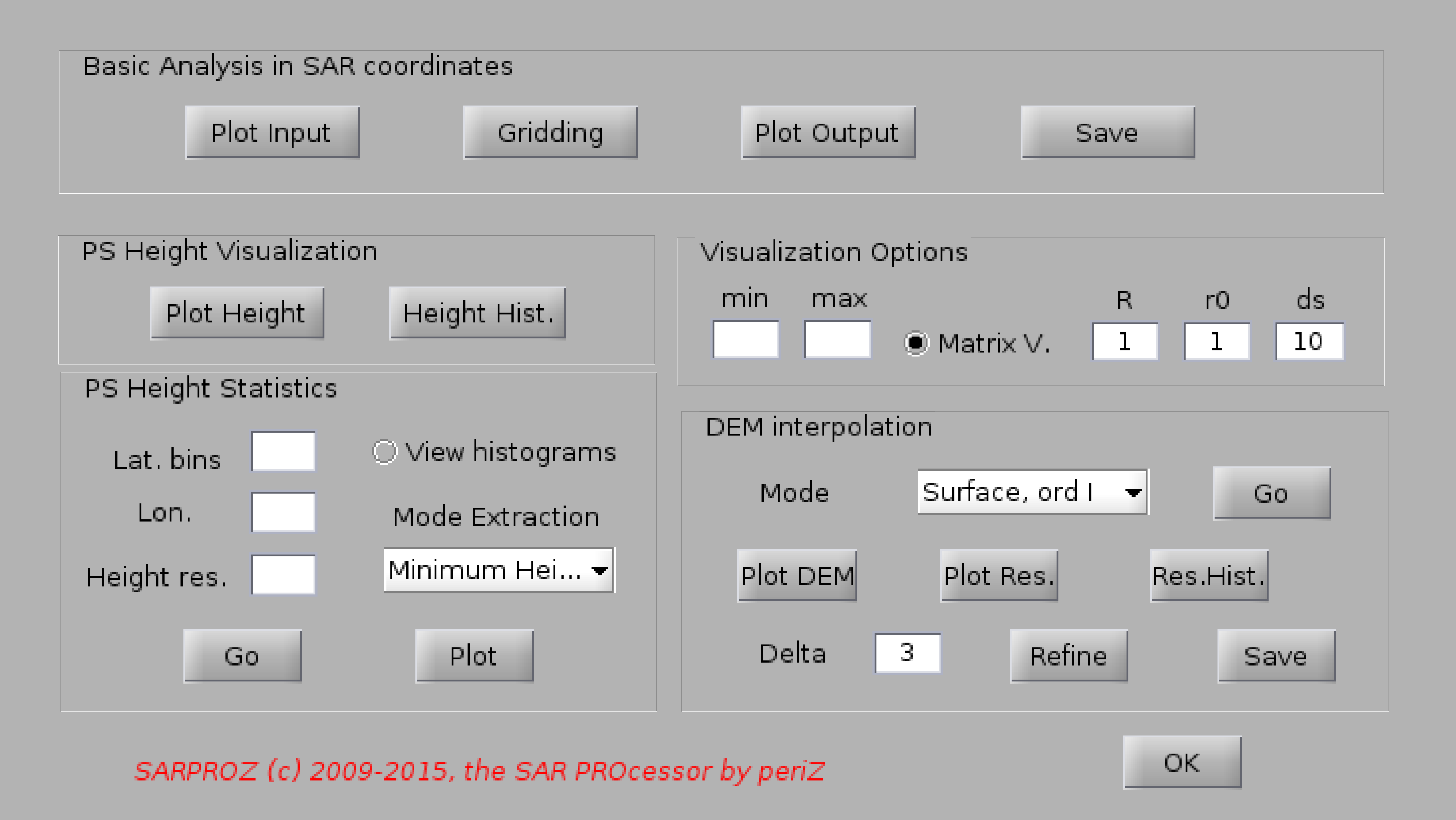
1.4.7.3. DEM Post-Analysis
Up
Help for DEM post-analysis
With this function you can post-process the height estimated with the multi-temporal InSAR analysis
for a sparse set of points in order to retrieve a digital elevation map of the are of interest.
In particular, this function has been written for extracting the height of the ground in urban sites
(Digital Terrain Model, DTM) [1,2]. However, you can use the following steps also for generating a common
DEM or a more advanced DSM.
Firstly, you can visualize the estimated height and its histogram using the 2 functions in the
"PS height visualization" box.
Then, you can analyze the height statistics in 3D with the functions in the panel "PS Height Statistics".
To achieve the aim, histograms are calculated by dividing the geographical space into "Lat bins" by "Lon bins" tiles.
The vertical sampling is defined by "Height Res".
The tool extracts a sample for each tile, according to the histogram modes. Currently, aiming at DTM estimation,
two modes can be extracted: the first mode (height with highest frequency) or the mode with lowest height.
When processing histograms, one can choose to visualize them by checking "View histogram". Such visualization
clearly slows down consistently the whole estimation, and can be stopped by pressing ctrl+c in the Matlab command prompt.
After the processing is conclude, the estimated modes can be plotted with the function "Plot".
After sampling the PS height according to its spatial statistics, such values can be interpolated in order to
reconstruct a reference surface for the whole area of interest. Choices are either fitting a mathematical surface
(first or second order), or using the griddata fucntion in Matlab.
Results can be checked by visualizing the estimated surface with "Plot DEM", the height residuals with "Plot Res."
and their histogram with "Res. Hist.".
Finally, results can be saved with "save" assigning a name to the generated file. Results are written in the directory
RESULTS in the main site folder.
[1] D. Perissin, F. Rocca, "High accuracy urban DEM using Permanent Scatterers", IEEE TGARS,
Volume 44, Issue 11, Nov. 2006 Pages: 3338 - 3347.
[2] D. Perissin, "Validation of the sub-metric accuracy of vertical positioning of PS's in C band",
IEEE GRSL, Vol. 5, No. 3, July 2008, Pages: 502 - 506.
Back to main index
1.4.7.4. PS Classification Up
Help for Target Classification
This module makes it possible to classify Urban Targets into 6 main typologies:
poles, dihedrals, trihedrals, roofs, floor gratings, fences.
See the reference for details.
Parameters have been set up through the Milan test site.
Alternating polarization images are needed for a reliable classification.
Reference
D. Perissin, A. Ferretti, "Urban target recognition by means of repeated spaceborne SAR images",
IEEE Transactions on Geoscience and Remote Sensing, Volume 45, Issue 12, December 2007, Pages: 4043 - 4058.
Back to main index
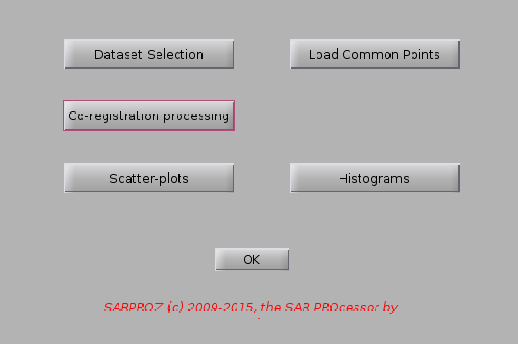
1.4.7.5. Multi-Sensor Analysis
Up
...description coming soon...
1.4.7.5.1. New Dataset Selection
1.4.7.5.2. Load Common Points
1.4.7.5.3. Fine Co-Registration
1.4.7.5.4. Scatter Plots
1.4.7.5.5. Histograms
Back to main index
1.4.7.5.1. New Dataset Selection
Up
...description coming soon...
Back to main index
1.4.7.5.2. Load Common Points
Up
...description coming soon...
Back to main index
1.4.7.5.3. Fine Co-Registration
Up
...description coming soon...
Back to main index
1.4.7.5.4. Scatter Plots
Up
Help for Scatter Plots under Multi-Sensor analysis.
For the different options of the plotting module, look at "Scatter Plots".
Here you can plot parameters coming from different sensors within the Multi-Sensor analysis.
To select a parameter from the secondary site, check the corresponding box "Track //" (this module was initially implemented for parallel tracks).
Back to main index
1.4.7.5.5. Histograms
Up
Help for Histograms under Multi-Sensor analysis.
For the different options of the plotting module, look at "Histograms".
Here you can plot histograms of parameters coming from different sensors within the Multi-Sensor analysis.
To select a parameter from the secondary site, check the corresponding box "Track //"
(this module was initially implemented for parallel tracks).
Back to main index
1.4.7.6. Cumulative Displacement
Up
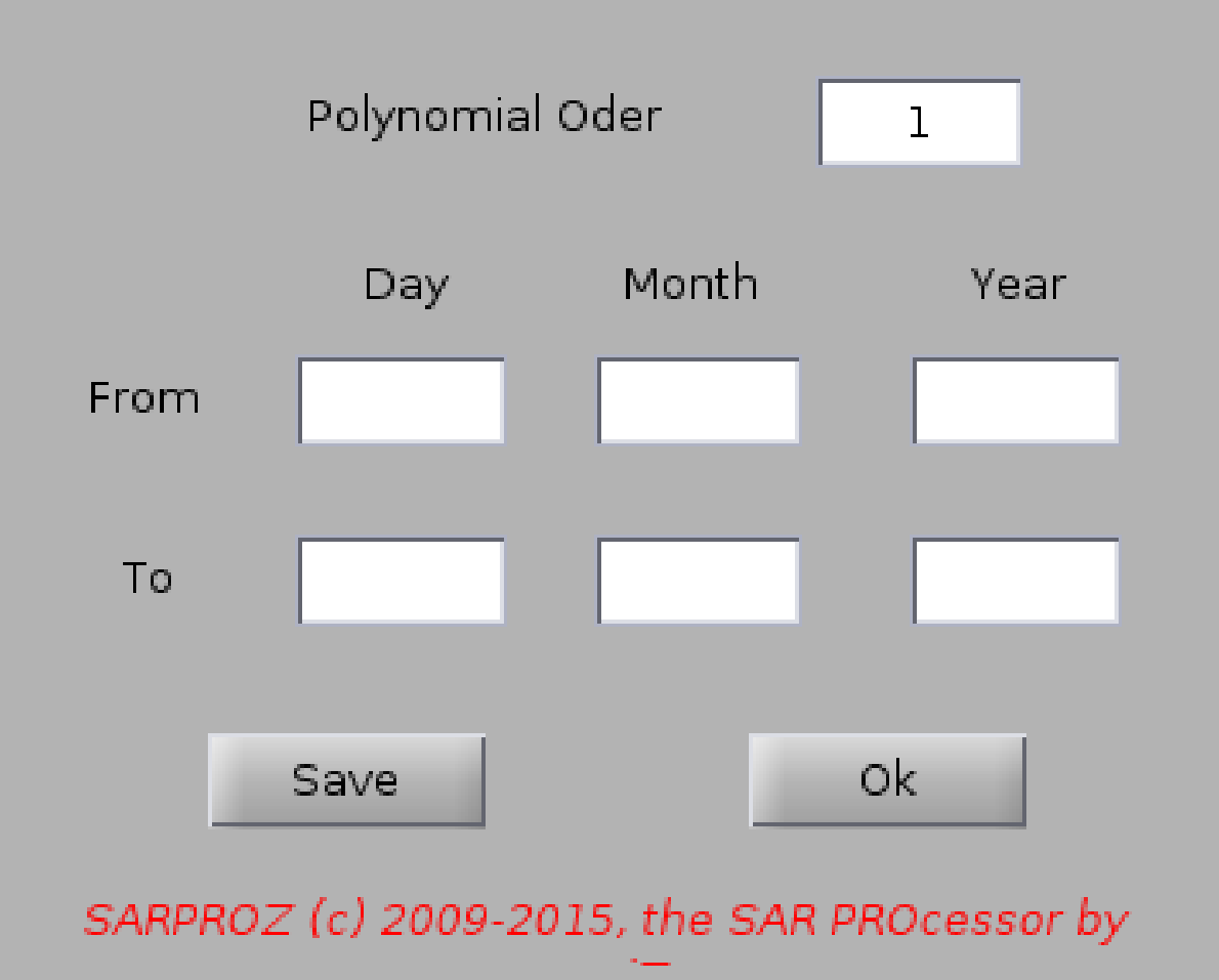
Help for Set Cumulative Displacement
With this function you can manually generate a file containing the cumulative displacement.
This function currently works only with polynomial models.
If you processed the time series through the "Sparse Points Processing", and you saved the
polynomial estimated coefficients, with this function you can read them and calculate
through the corresponding model the cumulative displacement between two given dates.
Note that the tool automatically saves a cumulative displacement calculated from the
beginning to the end of the loaded dataset.
Back to main index
1.4.8. Auxiliary Analysis Up
1.4.8.1. Change detection
1.4.8.2. Image classification
Back to main index
1.4.8.1. Change detection
Up
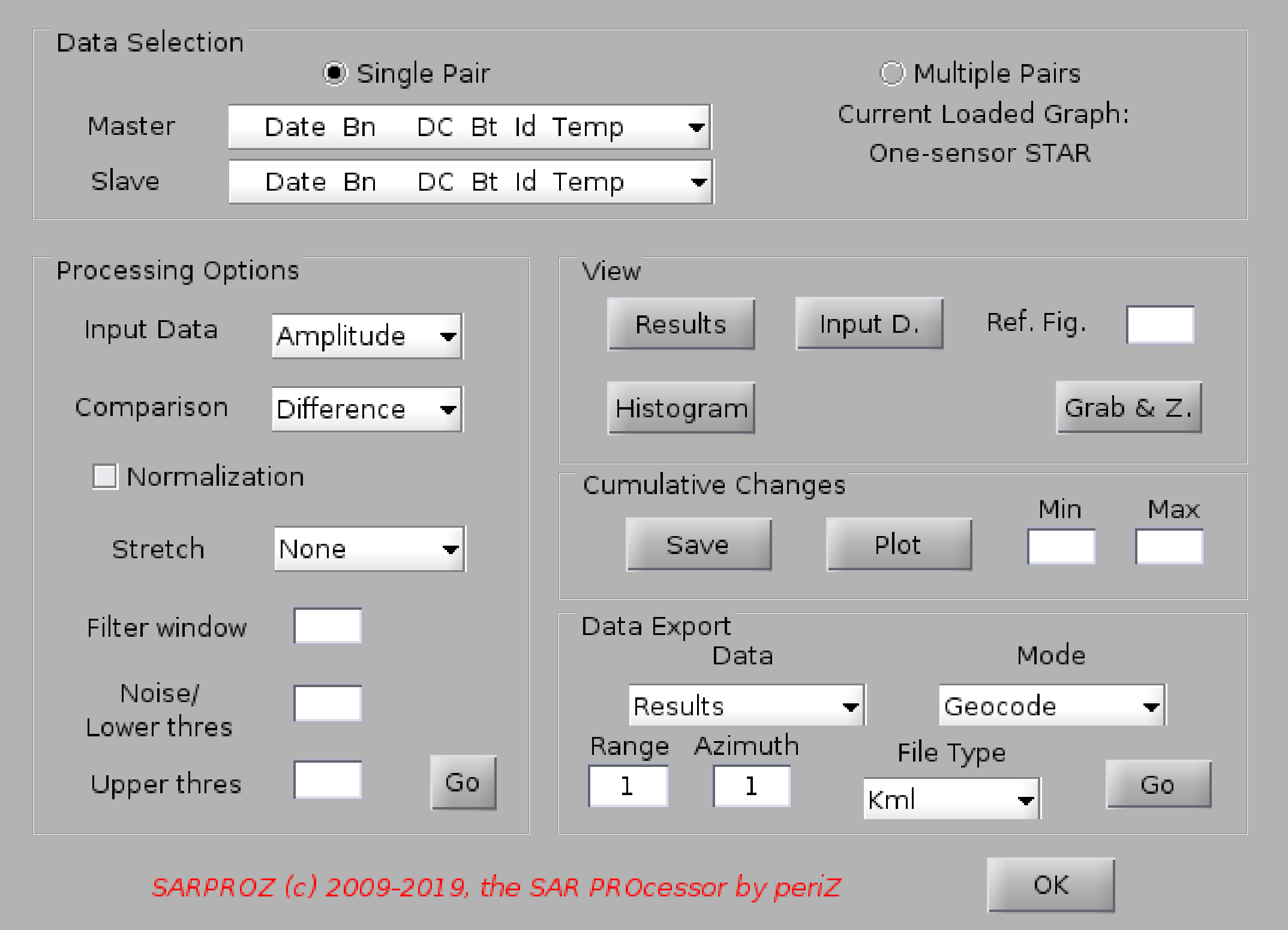
Help for Change Detection
...description coming soon...
Back to main index
1.4.8.2. Image classification
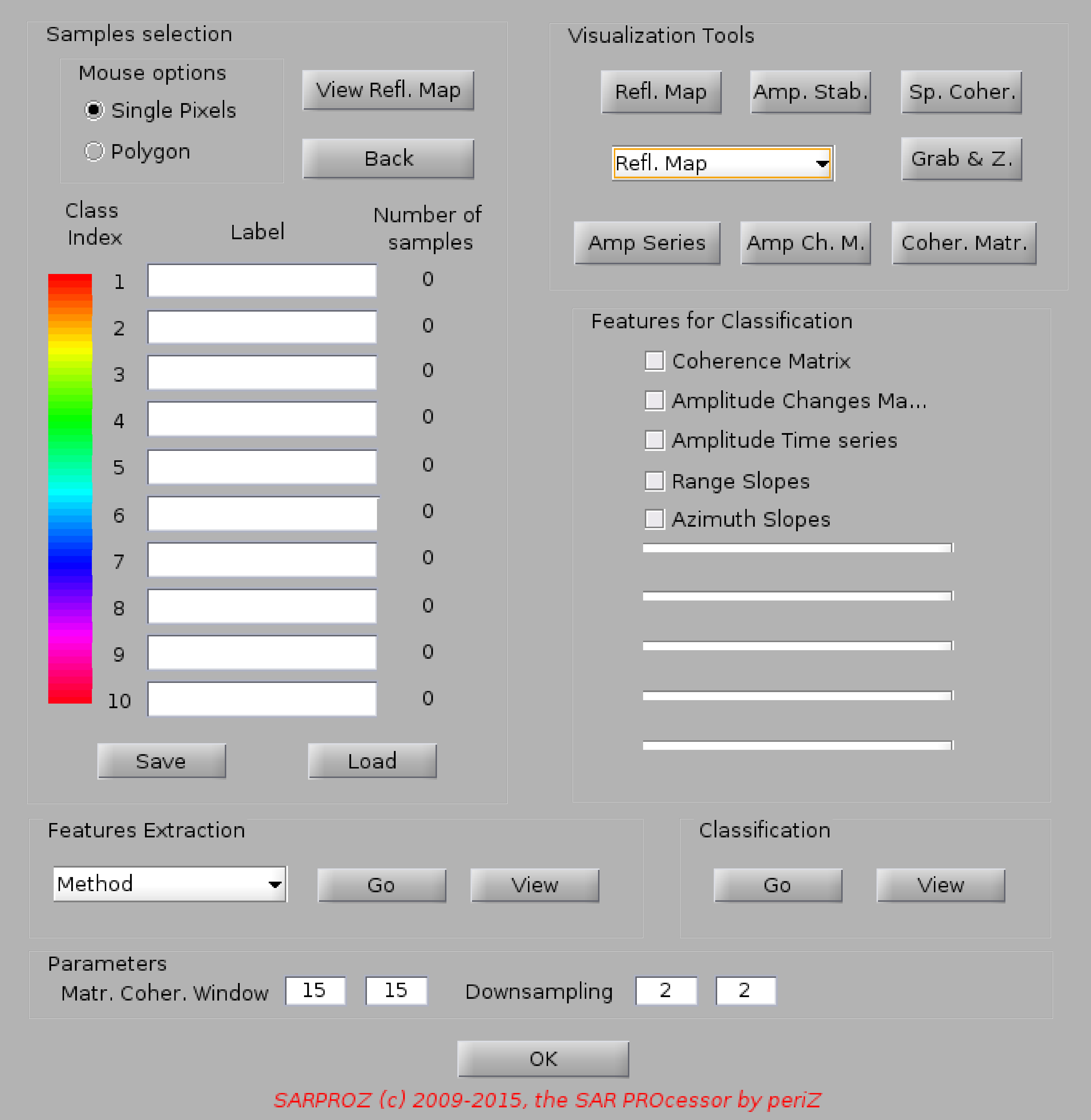
Help for Image Classification
Up
With this module you can firstly visualize a series of parameters for a selected pixel:
amplitude time series,
amplitude changes matrix,
amplitude coherence matrix.
Based on these observations, and on your knowledge of the anlyzed area, you can select a set of pixels belonging to different classes
(supervised classification), then you can select a series of features to characterize each class,
and then run a series of functions to classify all the area at hand.
The module is still under development and we be soon equipped by an unsupervised classification, based on data clustering.
Back to main index
1.4.9. Visualization Tools Up
1.4.9.1. Histograms
1.4.9.2. Scatter Plots
1.4.9.3. View Parameters
1.4.9.4. View Interferograms
Back to main index
1.4.9.1. Histograms
Up
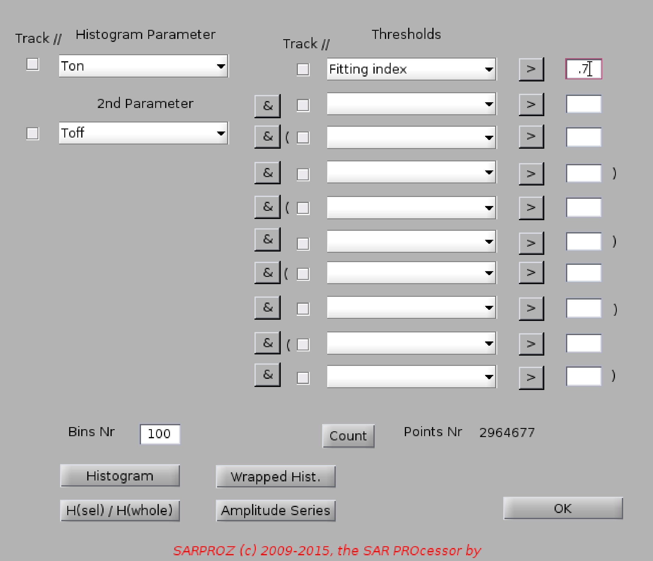
Help for Histograms
With this function you can plot histograms of all parameters managed by SARPROZ.
For the full list of parameters managed by SARPROZ, look at "Load Mask".
Select a parameter and press "Histogram".
To change the number of bins, specify the desired value in "Bins Nr".
You can plot till 2 parameters at a time, by choosing "2nd Parameter".
You can choose a subset of points for the histogram visualization
by filling the boolean selection conditions in the right columns.
Example of condition:
"Temporal coherence" > .8 & "Residual Height" < 20
In this way, all points with temporal coherence over .8 and residual height lower than 20
will be selected.
Press "Count" to apply the conditions. The number of selected points will be displayed.
By clicking on the corresponding signs, you can switch between and "&" and or "|" operators.
Note that there are pre-ordered brackets to group conditions.
Wrapped histograms can be plotted as well with a pie chart (clearly, this option has a meaning
when the parameter to be visualized is a phase).
Also a "relative" histogram can be displayed, showing the fraction between points selected with the above
conditions and the whole for each histogram bin.
Finally, to support the amplitude time series analysis, an options has been included to display
amplitude time series one by one for each point of the applied selection.
Back to main index
1.4.9.2. Scatter Plots
Up
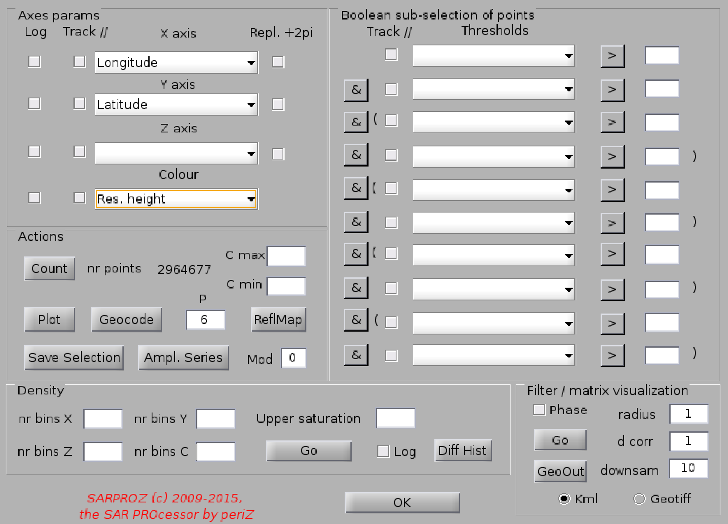
Help for Scatter Plots
With this function you can create plots of the parameters managed by SARPROZ.
For the full list of parameters managed by SARPROZ, look at "Load Mask".
Before launching this function, you have to select a sparse set of points that you want to analyze through the button
"Load Mask" in "Site processing".
You can create 2D and 3D scatter plots, colored 2D and 3D scatter plots, densities of scatter plots.
Finally, you can also visualize scatter plots in a matrix form (much quicker if you have many points to visualize).
Firstly, select the parameters to plot.
You can fill 4 axes: X, Y, Z and C, that stays for Color.
If you do not want to use one of the axes, leave it empty.
Depending on the chosen axes, a 2D or a 3D plot will be created, with or without a color code.
The plot is generate by clicking the button "Plot".
You can choose a subset of points for the plot creation
by filling the boolean selection conditions in the right columns.
Example of condition:
"Temporal coherence" > .8 & "Residual Height" < 20
In this way, all points with temporal coherence over .8 and residual height lower than 20
will be selected.
Press "Count" to apply the conditions. The number of selected points will be displayed.
By clicking on the corresponding signs, you can switch between and "&" and or "|" operators.
Note that there are pre-ordered brackets to group conditions.
Plotting Options:
You can saturate the color by the fields "C min" and "C max".
You can change the dot size through "P dim"
Auxiliary functions:
-------------------------------------------
"Geocode"
If you are displaying a parameter is SAR coordinates (Lines on X axis and sampled on Y axis), with this fucntion
you can grab the axes limits (the current displayed area) and launch automatically the small area geocoding module.
In this way, you can browse all parameters for the selected area. Advice: the area should not be too big to allow
the tool loading all results.
"ReflMap"
With this function you can plot the reflectivity map and superimpose the desired parameters on it.
To reach the aim, "X axis" must be "Lines" and "Y axis" "Samples".
"Save Selection"
You can save the selection operated with boolean expressions in a separate file and load it successively e.g from
"Load Mask".
This function will save the selection in a SAR coordinates file, samples by lines.
If a parameter on the C axis is selected, such parameter will be saved in the chosen file for the selected points.
"Plot Ampl. Series" and "Mod"
To support the amplitude time series analysis, this options has been included to display
amplitude time series for each selected point of the plot (use the Datacursor Matlab tool to select a point).
"Mod" refers to the amplitude series fitting model.
"Density"
Under this panel you can select several options to display the density of points of the scatter plot.
"Filter / Matrix Visualization"
...
1.4.9.2.1. Save Selection
Back to main index
1.4.9.2.1. Save Selection Up
Help for Save Selection in Scatter Plots
With this function you can save the selected set of points in Scatter Plots.
You will be asked to give a name to the file in which the selection will be saved.
The file is automatically saved in the RESULTS directory within the dataset directory.
In this way, you can re-select in a second time the same set of points simply selecting
"Choose file" from the Menu Selection (available at many steps of the tool)
and picking up the file you created.
Note: if a parameter for the Color information is selected, its content will be saved
for the current set of points. If no parameter is selected, ones will be written.
Back to main index
1.4.9.3. View Parameters
Up
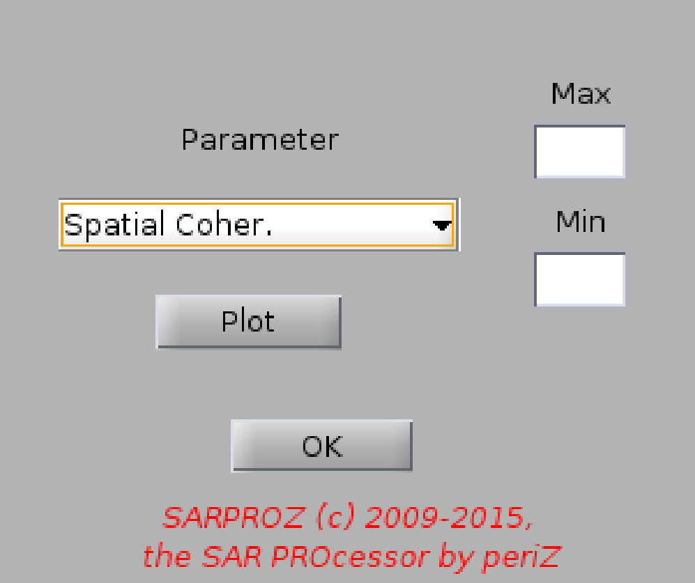
Help for View Parameters
With this function you can visualize parameters in SARPROZ.
For the full list of parameters that you can visualize, look at "Load Mask".
Parameters are here plotted in a matrix form.
For plotting parameters on a point basis, look at "Scatter Plots".
You can choose the saturation interval through the values "Min" and "Max".
Back to main index
1.4.9.4. View Interferograms Up
Help for View Interferograms
with this function you can plot the interferograms according to the images graph currently loaded and to the chosen InSAR parameters.
You can change the images graph in "Dataset Selection". InSAR parameters are changed via the "InSAR Params" button in "Site Processing".
Interferograms are plotted one by one. Both the phase and the coherence are displayed.
Back to main index
1.4.10. Results Exporting Up
1.4.10.1. Extended geocoding
1.4.10.2. Sparse geocoding
Back to main index
1.4.10.1. Extended geocoding
Up
Help for Extended Geocoding module
With this function the tool exports data and results in Google Earth format (kml and kmz).
In particular, under this module the tool exports matrixes of data, transforming SAR coordinates into
geographical coordinates.
For exporting data on a point-wise basis, refer to "Sparse geocoding".
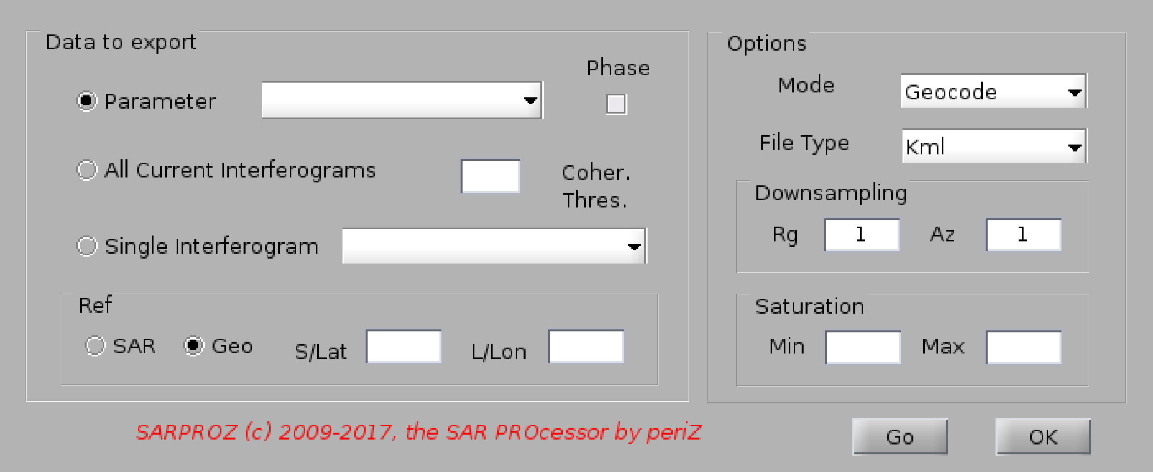
In this module, you can choose among 3 operations:
- geocoding a parameter (look at "Load mask for the full list of parameters")
- geocoding all existent interferograms (the tool will look for all files contained in the directory "INTERFEROGRAMS")
- geocoding a single interferogram among those listed in the menu (corresponding to the currently loaded images graph)
Finally, one can choose to downsample the data through the inputs "Range" and "Azimuth".
Back to main index
1.4.10.2. Sparse geocoding
Up
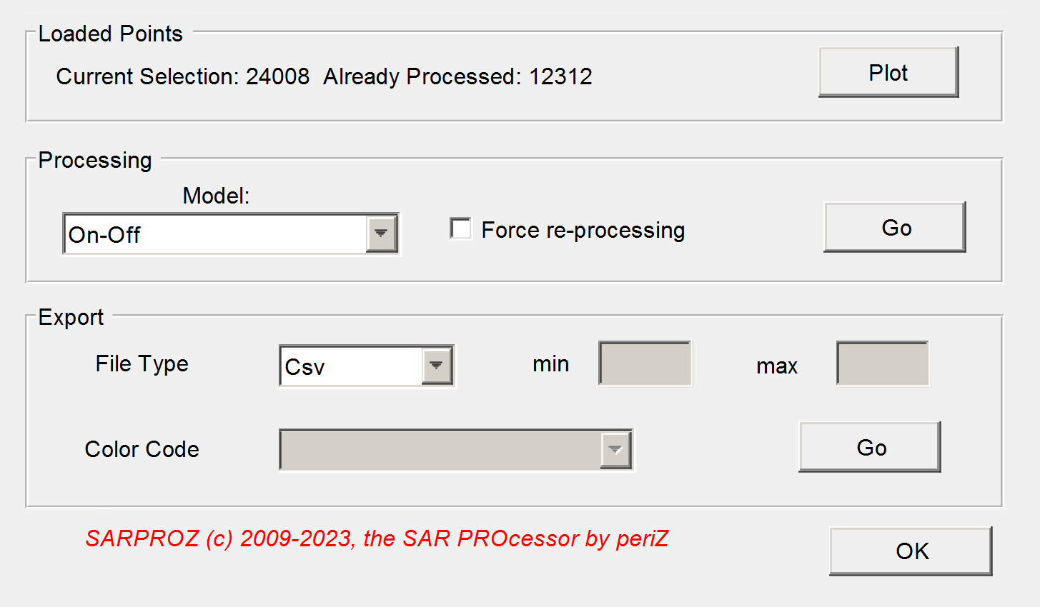
Help for Sparse Geocoding
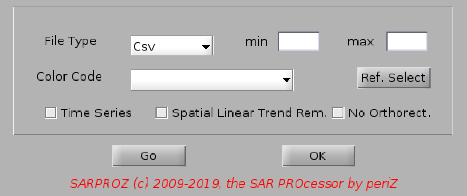
With this fucntion, the tool exports data on a point-wise basis.
Data can be exported in 3 main formats:
- dbf files (text tables in dbf format)
- kml files (Google Earth extension)
- 3D kml files (Google Earth extension)
Data are color-coded according to the selected parameter ("Color Code").
Look at "Load Mask" for the full list of parameters.
The color can be saturated passing minimum and maximum values ("min" and "max").
A spatial linear trend can be removed by selecting the corresponding check-box.
A reference point can be selected as well (should have been saved by the "APS estimation" module).
Default reference point is automatically selected.
Finally, time series can be included in the exported data by selecting the corresponding check-box.
This last operation is a bit time consuming (depending on the set of selected points) since the tool
reads from the disk all the data time series from the original SAR images.
Back to main index
1.4.11. Sub-dataset Extraction Up
1.4.11.1. Selection and Extraction
Back to main index
1.4.11.1. Selection and Extraction
Up
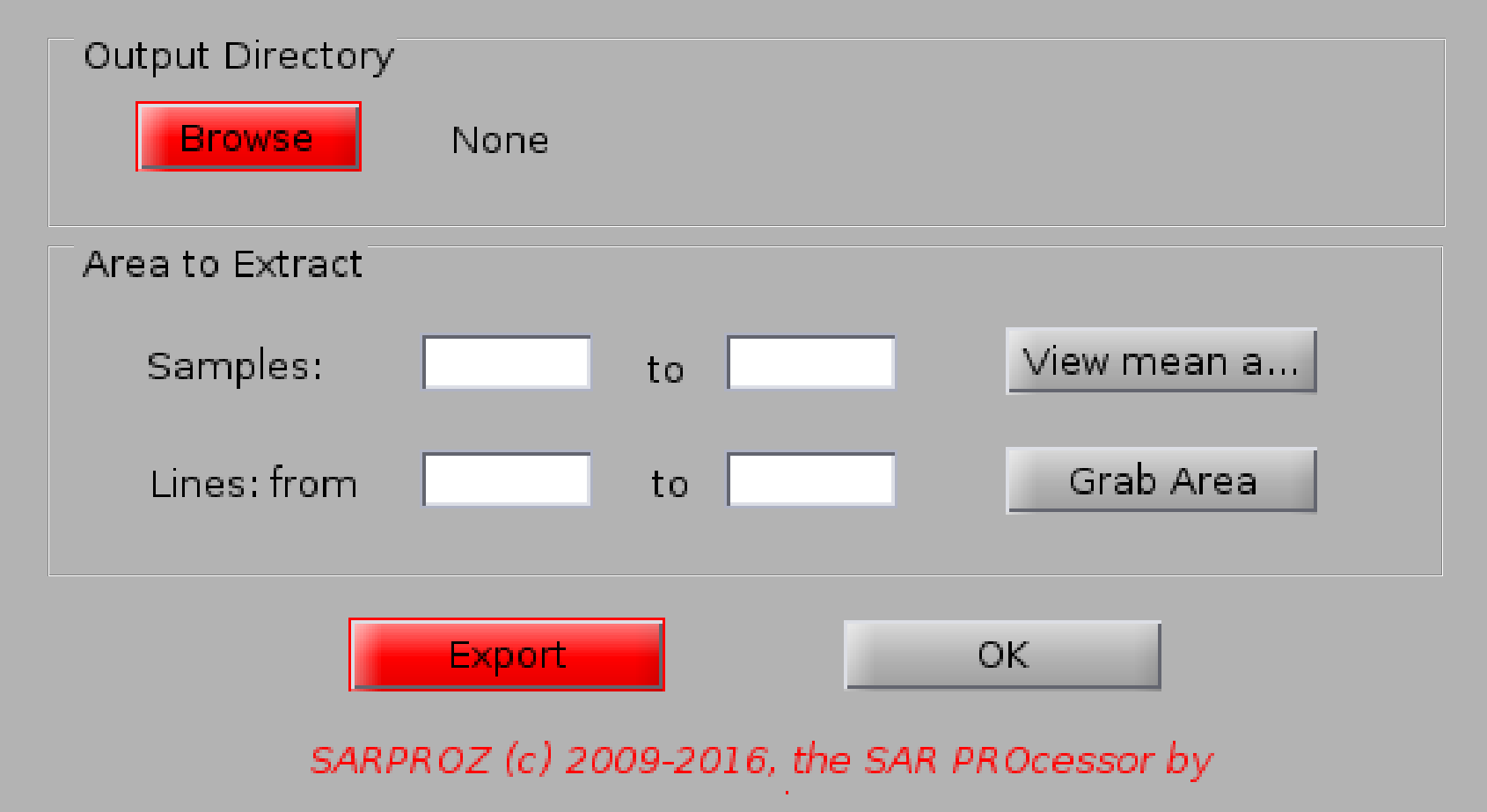
Help for sub-set dataset extraction
Use this function to select a small area and to create a corresponding new dataset.
Back to main index
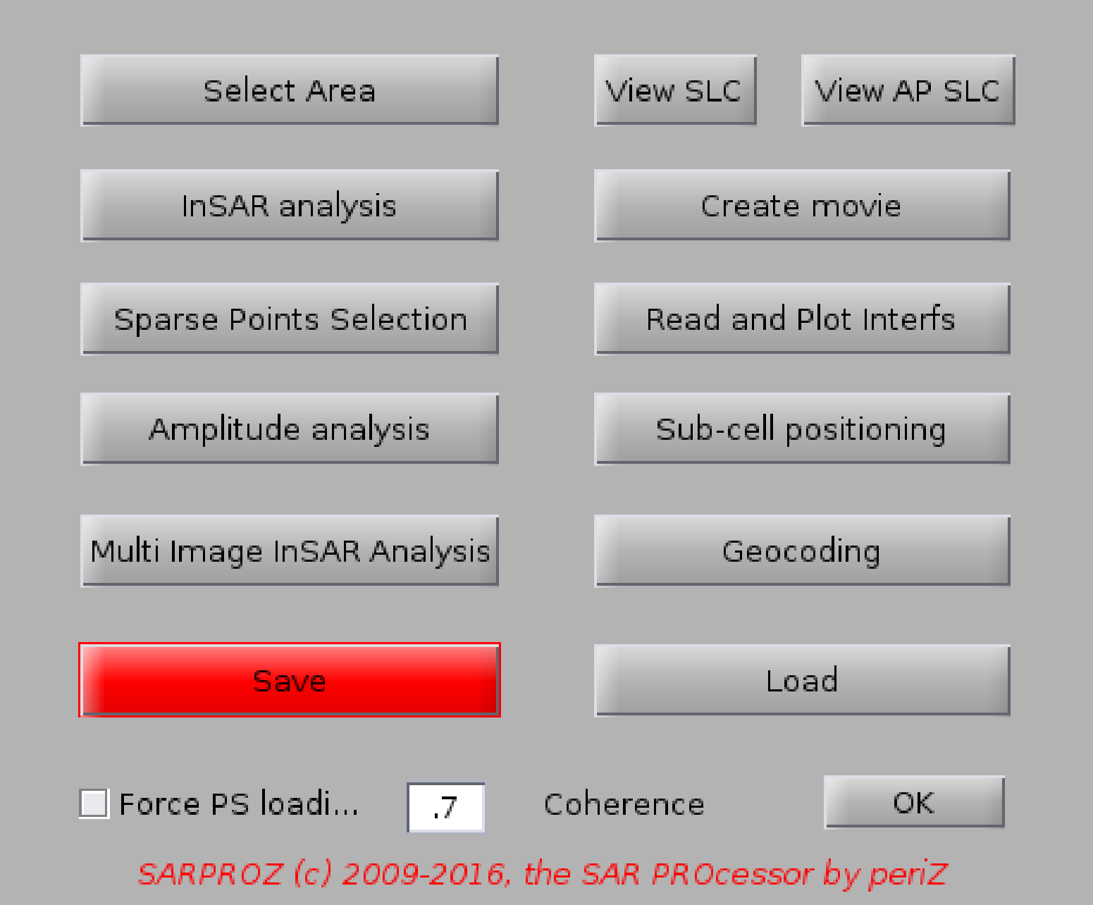
Help for Small Area Processing
This module of the tool starts an independent processing session.
The core idea is to process a small area to analyze it in depth or
to quickly test different techniques.
The module can be used for teaching the basics of InSAR and PSInSAR
as well as more advanced functions.
This module is available in the Demo version, but it can be used only with pre-processed data.
The module includes a function for selecting the area to process,
a basic visualization of each image (with the possibility of creating a movie of the images amplitude),
a sub-module for InSAR analysis,
a sub-module for processing amplitude time series,
a sub-module for PSInSAR-QPSInSAR processing
a module for geocoding the results, visualizing them on an optical layer, ploting all parameters and time series.
Finally, it is possible to save the work-space in a matlab file. In this way, you can load it in Sarproz later on again
and go on processing it without loosing what was already done. Moreover, you can also load the workspace directly in Matlab
and apply your own algorithms.
Furhter help can be seen in each sub-module.
1.5.1. Select area
1.5.2. View SLC
1.5.3. View AP SLC
1.5.4. Create Movie
1.5.5. S.A. InSAR analysis
1.5.6. S.A. Amplitude analysis
1.5.7. S.A. Sub-cell positioning
1.5.8. S.A. Multi image InSAR analysis
1.5.9. S.A. Geocoding
1.5.10. Save
1.5.11. Load
Back to main index
1.5.1. Select area
Up
Help for Select Area
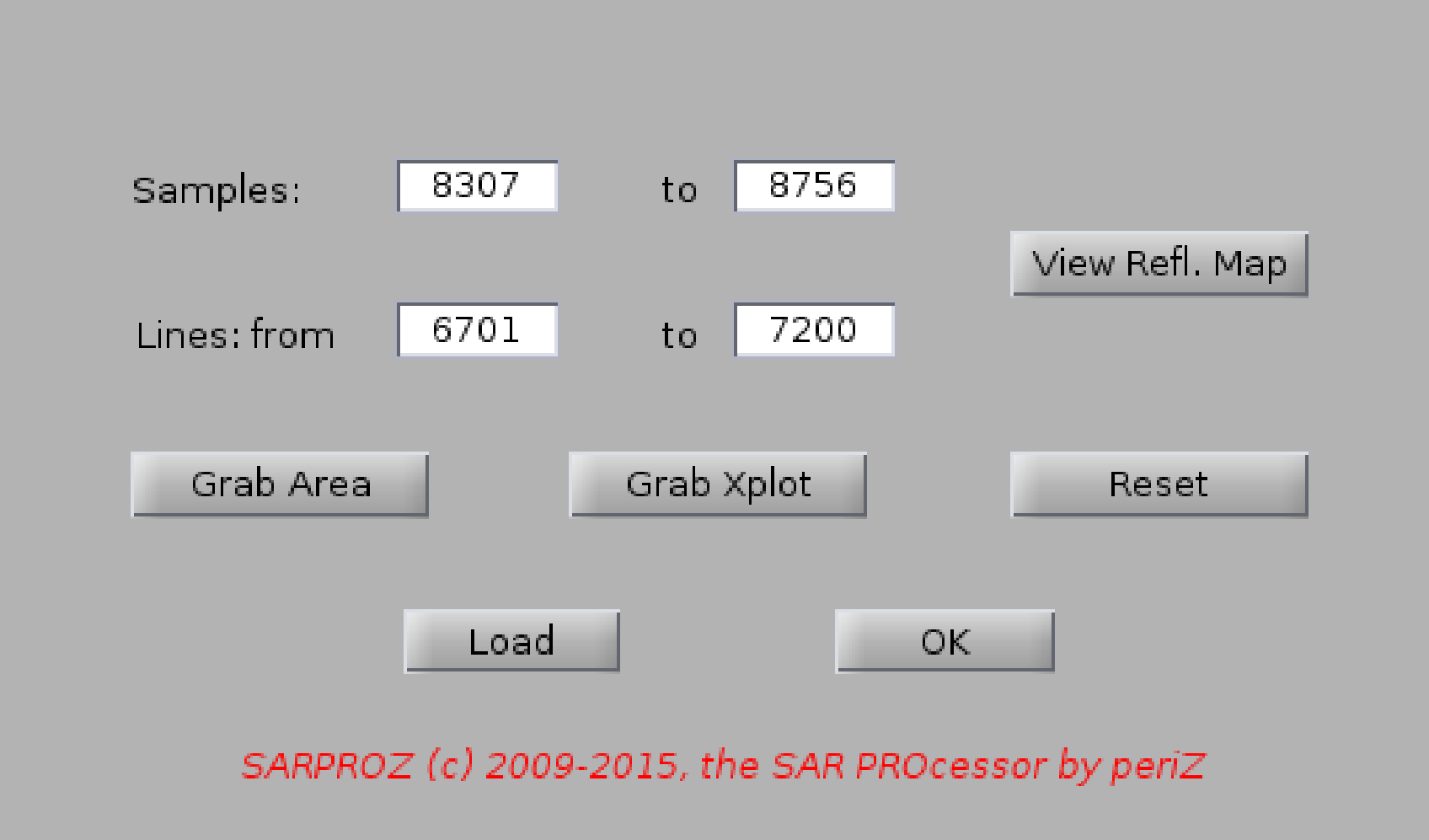
With this function you can select a small area to process.
The area can be selected either by inputing the range and azimuth pixels to extract
or by plotting the Reflectivity Map ("View mean amplitude"), zooming on the desired area,
an then clicking "Grab Area". This button automatically extracts the bounds of the imaged area.
Finally, it is possible to use this function together with the function "Scatter Plots" in Site Processing,
and select the area zoomed in the window generated by Scatter Plots.
By pressing OK, the tool loads all data relative to the choosed area.
Back to main index
1.5.2. View SLC Up
Help for View SLC
This function plots sequentially amplitude and phase of all images of the dataset, according to the
small area selected.
To view the next image, click the button "Go" on the window "Take a Decision", that opens after
visualizing an image.
By clicking "Stop" the sequence is stopped and all windows closed.
Tip: arrange as you like the images and consider that the window "Take a Decision" will be open newly in the same position at the
next iteration.
Back to main index
1.5.3. View AP SLC Up
Help for View AP SLC
this OBSOLETE function was implemented to look at the AP images of the DataSet.
It needs to be generalized in case of need.
Back to main index
1.5.4. Create Movie Up
Help for Create Movie
With this function you can create a movie of the amplitude of the SAR images.
The name of the generated file will be displayed on the command prompt.
Back to main index
1.5.5. S.A. InSAR analysis
Up
Help for InSAR Analysis module
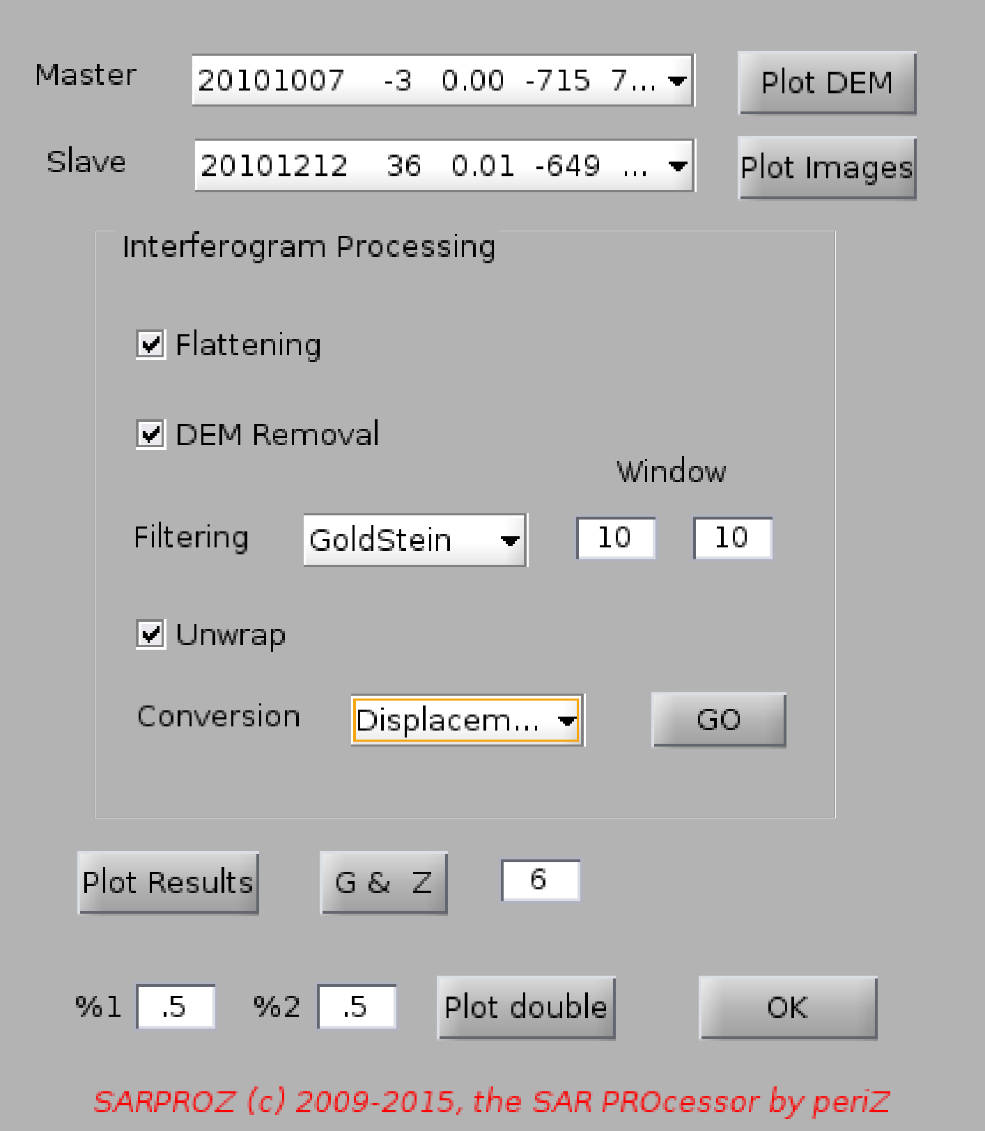
In this module, you can perform the basic functions for InSAR processing.
Firstly, select Master and Slave images by clicking the corresponding menu.
Note that for each image a list of parameters is shown.
In sequence: image date, Normal Baseline, Doppler Centroid, Temporal Baseline,
a number identifying the Sensor, Temperature.
By clicking "Plot Images", you can visualize amplitude and phase of the corresponding pair.
With "Plot DEM" you can see the DEM in the selected area.
Choose the operations to perform on the selected images pair:
-Flat terrain phase term removal
-Topographic phase term removal removal
-Filtering (at the moment you can choose among BoxCar, modified Goldstein, median),
for which you can specify the window size
-Unwrapping
-Phase conversion (into m -topography- or mm -displacement-).
Then click "GO" and the selected operations will be applied
You can then see the interferogram, coherence image and histogram by means of "Plot Results".
"G & Z" stays for Grab and Zoom. If you are looking at some details in the interferogram
(shown in Figure 6), write "6" beside "G & Z" and click it: all open images will be zoomed
on the same details.
"Plot Double" shows the colored interferometric phase superimposed on the interferogram
amplitude (black and white). You can choose a percentage of transparency of both values.
Back to main index
1.5.6. S.A. Amplitude analysis
Up
Help for Small area Amplitude analysis
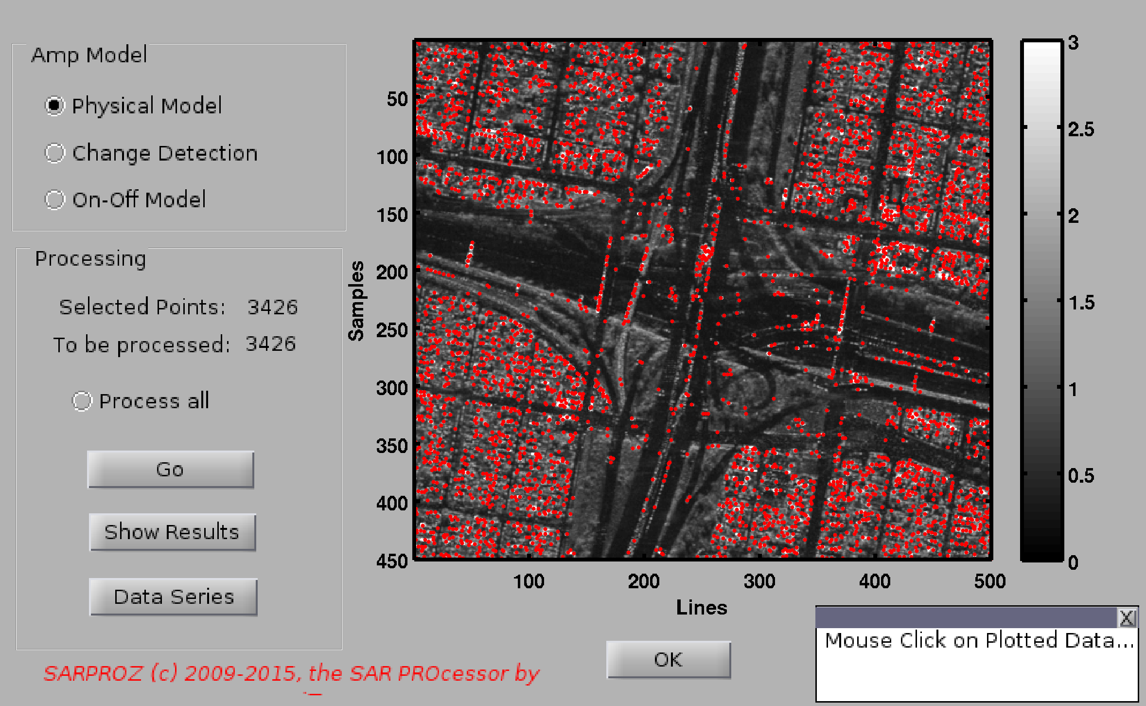
With this function you can firstly select a set of points to process within the analyzed area.
You can select sparse points in two ways:
-either by choosing a parameter and posing a threshold (see "Load mask" in "Site processing" for more advanced explanations)
-or by posing a threshold on the Amplitude and then choosing whether extracting Local Maxima and/or Side Lobes
The selected points are visualized on the reflectivity map beside.
After selecting points, you can choose to process the amplitude time series by pressing the "Go" button.
For details on the analysis, check the help for "Amplitude time series analysis" in "Site processing".
After processing, a window will be opened showing the results. You can choose to review the results one by one by clicking "Next",
quitting by clicking "Exit" or processing again the current result by clicking the corresponding button.
Alternatively, you can view the estimated parameters by clicking "Show Results" or the time series of each target by clicking
"Data Series".
You can also choose NOT to process the amplitude time series and quit after selecting the set of sparse points.
The tool will ask for confirmation.
Back to main index
1.5.7. S.A. Sub-cell positioning Up
Help for Sub-cell positioning
With this function, the sub-cell position of each scatterer is calculated by processing
the amplitude of nearby pixels in each image. Basically, the position of the peak of
a cardinal sine fitting the data is extracted.
Then, the sub-cell position in each image is plotted as a function of Time, Normal Baseline
and Doppler Centroid for each target.
Press Enter on the command prompt to view the plots of next target or press "q" Enter to terminate.
Back to main index
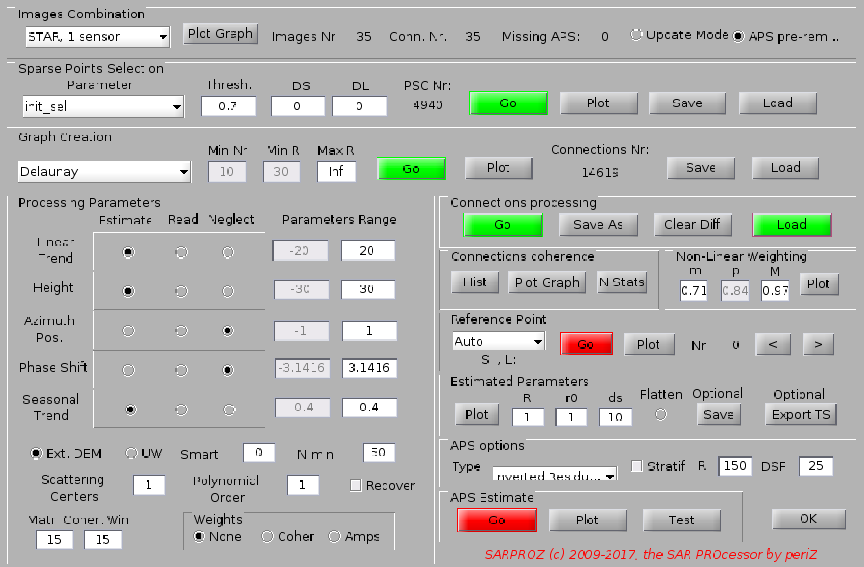
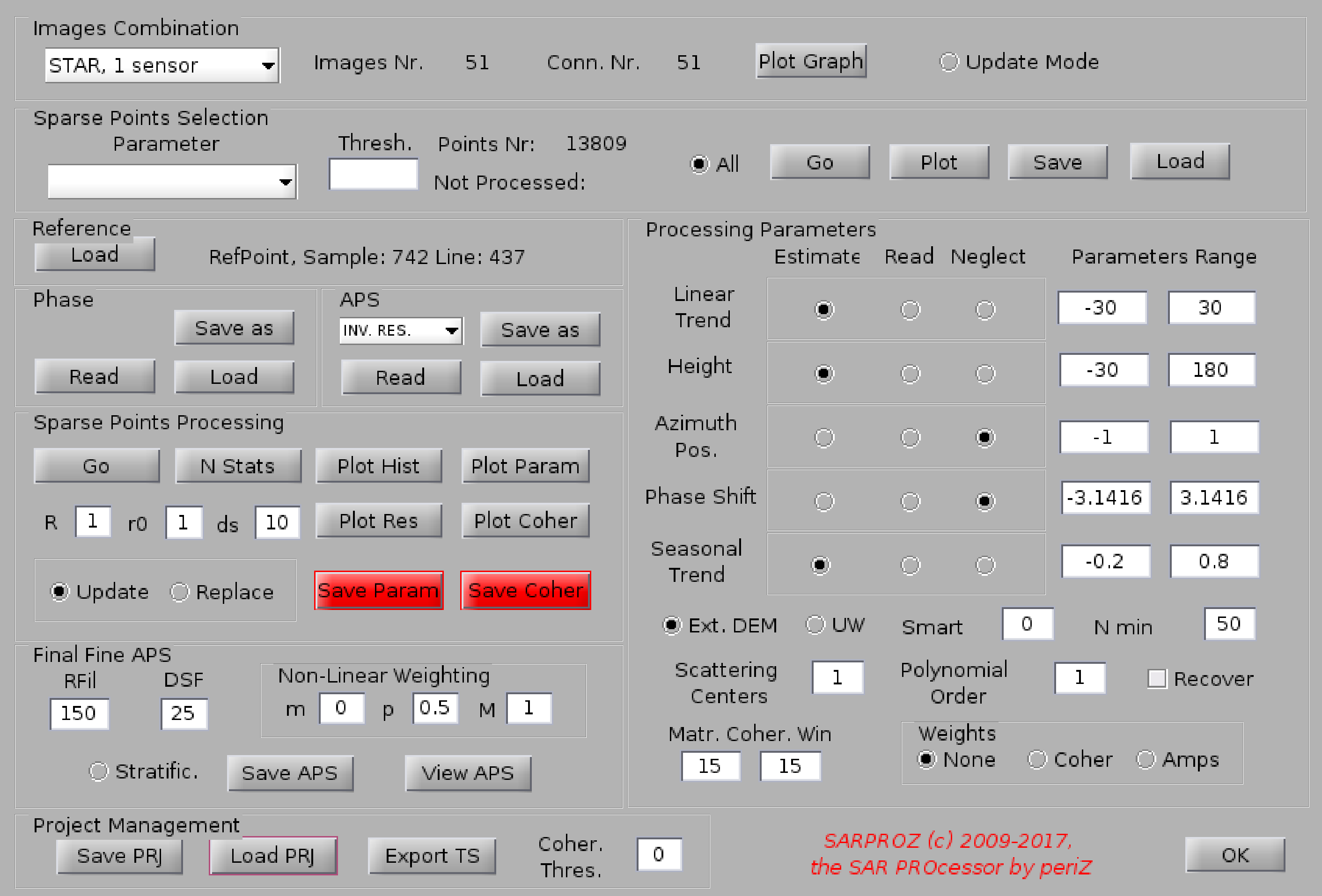
1.5.8. S.A. Multi image InSAR analysis
Up
Help for Small Area Sparse Points Multi-Image InSAR Processing Module
This module performs Sparse Points Multi-Image InSAR processing for a small area.
Which points to process has to be previously chosen by means of the Amplitude Analysis module.
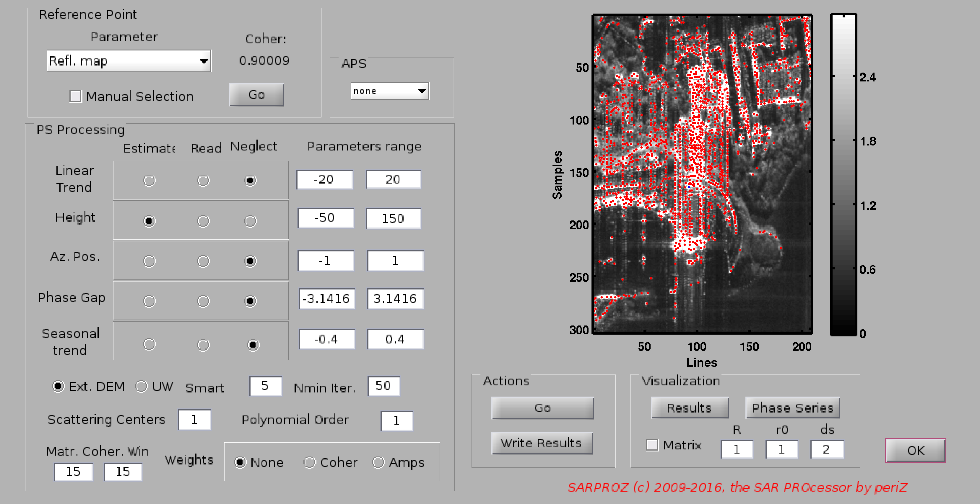
Reference selection/ APS compensation
The PS processing module allows to choose a Reference point by selecting a parameter to maximize.
The Reference point is plotted in blue color on the reflectivity map.
If the parameter is left empty, a best choice is applied considering the interferograms derived by the current Images Graph.
Then, whether to compensate for the previously estimated APS can be chosen.
In alternative, one can decide to compensate for the error introduced by the noise of the reference point.
Phase processing
After chosing reference point and APS compensation, phase time series are analyzed.
Five parameters can be either estimated, or compesanted for (if previously estimated) or neglected:
-Linear trend
-Height
-Azimuth Position (in case of Doppler Centroid variability)
-Phase Gap (in case of different carrier frequencies)
-Seasonal Trend
Moreover, the external DEM can be subtracted from the phase series by flagging "a priori DEM".
Phase time series are generated according to the images graph selected in the Main window
(star graph with a unique Master image, or MST, or Full Graph...)
Phase time series can be weighted by means of the spatial coherence of corresponing interferograms
by flagging "weights". If interferograms are not available, the coherence matrix is processed.
Finally, the processed results can be plotted ("Show Results"), together with Phase Time Series ("Phase Series").
The results can be written in the corresponding full site matrixes with "Write Results".
Back to main index
1.5.9. S.A. Geocoding
Up
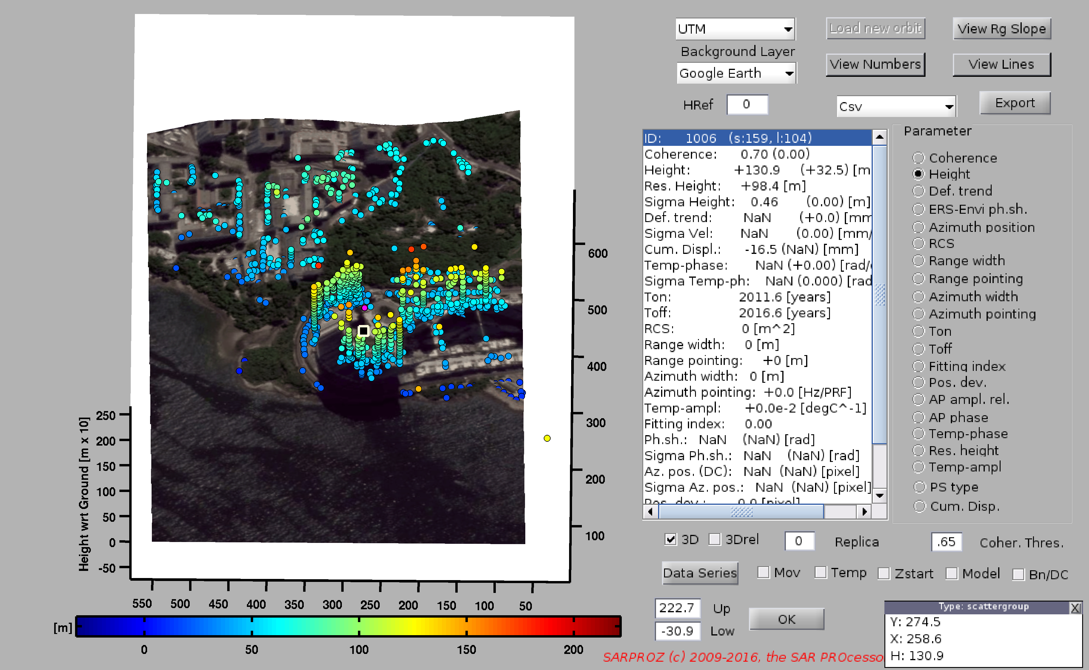
Help for Small Area Geocoding
This module performs the visualization of PS analysis carried out in the small area.
PS are plotted in UTM coordinates.
An optical layer can be selected and displayed as background by means of the "layer" button (geocoded TIF can be loaded).
PSs are plotted with a color scale that can be used to visualize the estimated parameters.
You can switch amoung parameters by clicking the list on the right.
The colorbar can be saturated by specifying upper and lower values.
PS can be plotted in 3D coordinates ticking the "3D" box.
The box "3Drel" uses the height relative to the external DEM as vertical coordinate.
By specifying a "Coher. Thresh." only PSs over the threshold are displayed.
By using the Matlab "Data Cursor" tool (default tool when the window is opened),
and by clicking on a desired PS, the list of estimated parameters is shown.
Among brackets the parameters estimated in the whole site (if available) are reported (otherwise NaN is shown).
When a PS is selected, its phase time series can be displayed by clicking "Data Series".
By clicking "Data Series", the residual phase is plotted as a function of Time.
Together with phase, also the amplitude is plotted. The amplitude series show also the estimated model that fits the data.
To display the time series including the estimated movement component, tick the "Mov" box.
To display the time series including the estimated component correlated with temperature, tick the "Temp" box.
To force time series starting from zero in the first image, tick the "Zstart" box.
To plot also the estimated time-model, tick the "Model" box.
To display phase as a function of Normal Baseline and Doppler Centroid, tick the "Bn/DC" box.
The estimated parameters can also be exported in csv format clicking the "Csv" button.
Time series are exported according to the same options selected for data series plot (Mov, Temp, Zstart, Model, Nr of replica)
The csv file has a header indicating the exported parameters.
The first NI dates include the phase values in millimiters. Then replicas may come (notice that 1 replica corresponds +2pi and -2pi, that is, 2NI data more).
Finally, NI values for the model (if selected).
The options with which the csv was generated are reported in the first csv line.
Back to main index
1.5.10. Save Up
Help for Save in Small Area processing.
With this function you can save the workspace of the small area you are working on for loading it again at a second time.
All the currently processed results will be saved, together with a jpeg image showing the analyzed area.
Results are by default saved in a subdirectory of the dataset.
Back to main index
1.5.11. Load Up
Help for Load in Small Area processing.
with this function you can load a previously saved workspace relative to a small area.
By default, the tool looks in the associated dataset subdirectory.
Back to main index