Help for Small Area Geocoding
This module performs the visualization of PS analysis carried out in the small area.
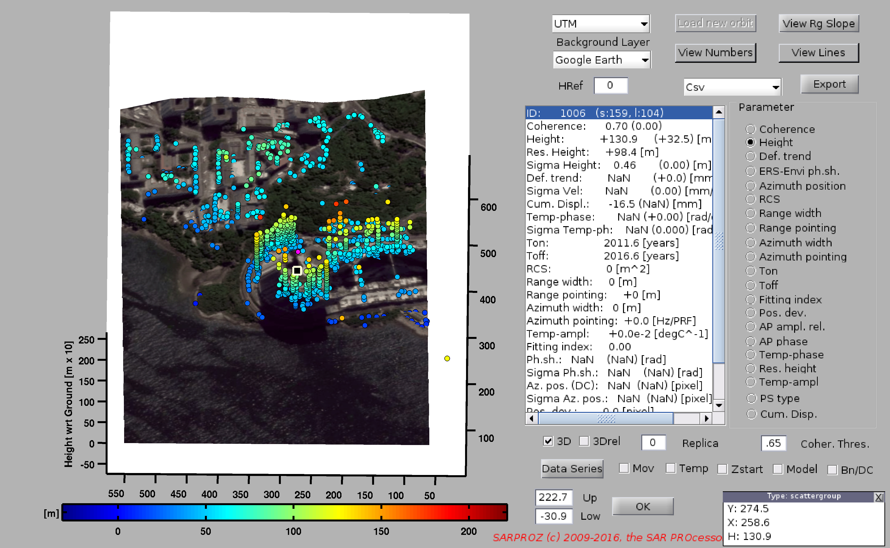
PS are plotted in UTM coordinates.
Different layers can be loaded as background with the corresponding menu:
- none (blank)
- Google Earth (an image is automatically downloaded)
- Reflectivity Map
- External DEM
- Select Dir (the sw will search for geotiff files)
PSs are plotted with a color scale that can be used to visualize the estimated parameters.
You can switch amoung parameters by clicking the list on the right.
The colorbar can be saturated by specifying upper and lower values.
PS can be plotted in 3D coordinates ticking the "3D" box.
The box "3Drel" uses the height relative to the external DEM as vertical coordinate.
By specifying a "Coher. Thresh." only PSs over the threshold are displayed.
By using the Matlab "Data Cursor" tool (default tool when the window is opened),
and by clicking on a desired PS, the list of estimated parameters is shown.
Among brackets the parameters estimated in the whole site (if available) are reported (otherwise NaN is shown).
When a PS is selected, its (LOS) phase time series can be displayed by clicking "Data Series".
By clicking "Data Series", the residual phase is plotted as a function of Time.
Together with phase, also the amplitude is plotted. The amplitude series show also the estimated model that fits the data.
To display the time series including the estimated movement component, tick the "Mov" box.
To display the time series including the estimated component correlated with temperature, tick the "Temp" box.
To force time series starting from zero in the first image, tick the "Zstart" box.
To plot also the estimated time-model, tick the "Model" box.
To display phase as a function of Normal Baseline and Doppler Centroid, tick the "Bn/DC" box.
The estimated parameters can also be exported in different formats:
- Csv
- Jpegs
- kmls (2d, absolute 3d, relative 3d)
by choosing the corresponding option from the mene and by clicking "export"
Time series are exported according to the same options selected for data series plot (Mov, Temp, Zstart, Model, Nr of replica)
The csv file has a header indicating the exported parameters.
The first NI dates include the phase values in millimiters. Then replicas may come (notice that 1 replica corresponds +2pi and -2pi, that is, 2NI data more).
Finally, NI values for the model (if selected).
The options with which the csv was generated are reported in the first csv line.
If the reference point was not previously processed in the full site, its height may not be precise and the points will be shifted along the range.
To correct such a shift, you can input a number in the HRef box and the points will be shifted accordingly.
Trick for resetting the geocoded images: write "reset" in the "Href" box.
To display the Line Of Sight of the satellite, click on "View Lines".
To display the ID number of each point, click on "View Numbers".
To display the Line Of Sight of the satellite together with the range slope, select a point in the map and click on "View Rag Slope".