Help for Single Interferogram Processing
With this function you can choose freely one interferogram to process and visualize.
You can also process a smaller area and choose which operations to perform.
Steps to follos and options to choose:
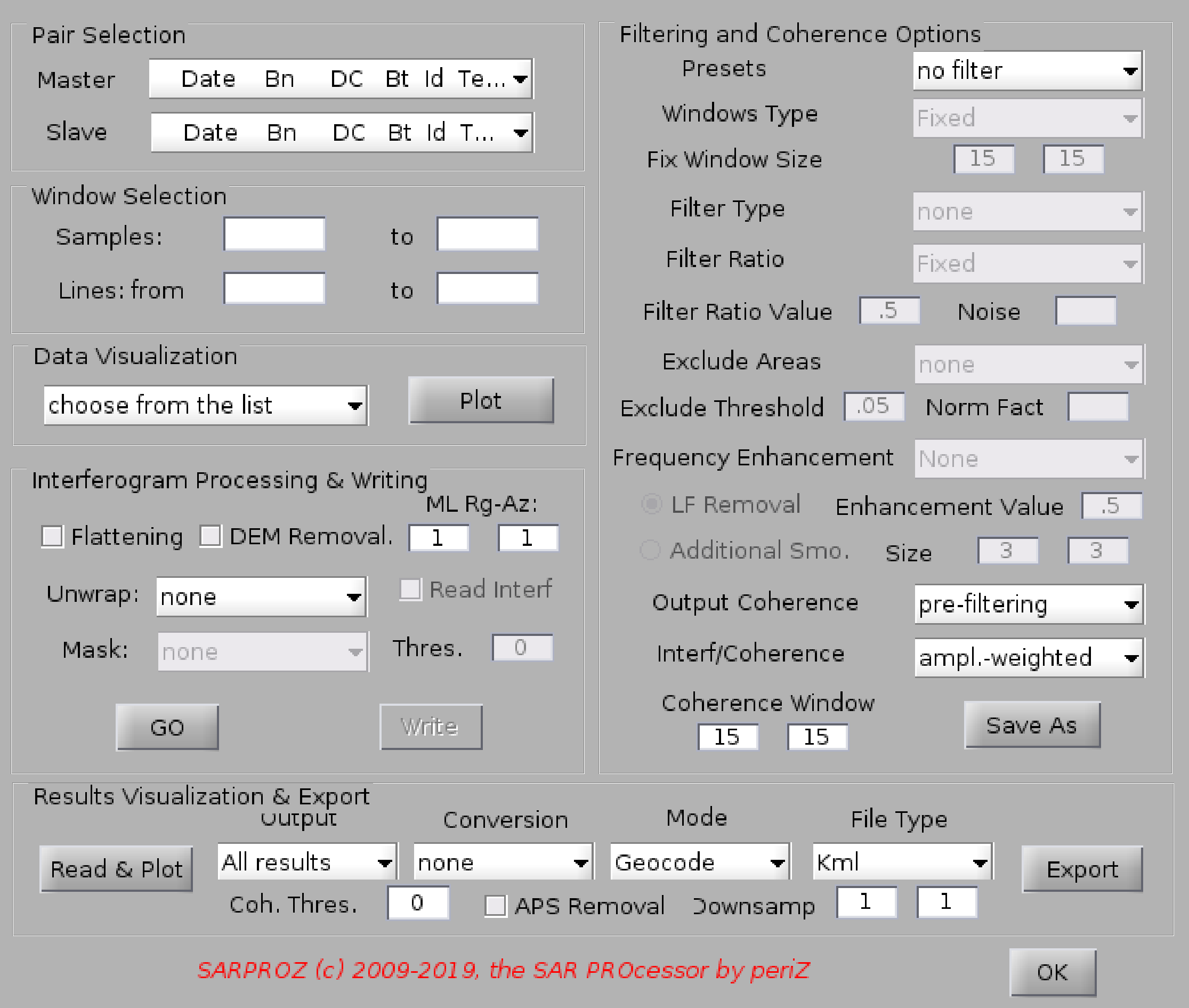
1. select the pair of images to process (master/slave). For each image, data, Normal Baseline, Doppler Centroid, Temporal Baseline,
Satellite Id and Temperature are displayed. Relative values are referred to the Master image.
2. (optional) you can choose a small area for focusing on some details or for testing different options in a short time. Just specify
starting and ending samples and lines
3. you can visualize the data before processing. Current data available for visualization are: absolute values of Master and Slave,
DEM, Local Mususigma, local variance, histograms of absolute values of Master and Slave. Noitce that Local Mususigma and local variance
are calculated using the options specified in the filtering option panel (windows type, windows size, filter type)
4. choose whether to remove or not flat terrain phase and topographic phase
5. choose whether to multi-look your interferogram
6. choose whether to unwrap the interferogram (additional options for unwrapping: mask for escluding any given area, conversion to meters/millimeters)
7. choose the filtering options (filtering and coherence options panel)
- some predifined options are available from the presets menu:
* no filter (no further options)
* boxcar (you can choose the window size)
* goldstein (you can choose window size and fixed frequency enhancement coefficient)
* modified goldstein (you can choose the window size)
* multi-temporal adaptive
* single-interferogram adaptive
* Wiener (you can choose the window size and the optional noise level)
* custom filter (all options available)
* load options (you can load a previously saved options file)
- windows type:
* fixed (you can choose the size)
* adaptive (based on the multi-temporal mask)
* adaptive (based on single interferogram statistics)
- fix window size
- filter type:
* none
* moving average
- filter ratio:
* fixed (it works as a common filter, you can set the filter ratio value)
* mususigma (it weights the filtering effect according to the local mususigma vs noise: mususigma>noise --> don't filter. mususigma
* localvar (it weights the filtering effect according to the local variance vs noise: variance>noise --> don't filter. variance
* local coher (it weights the filtering effect according to the local coherence: coherence>noise --> filter. coherence
- filter ratio value: you can set it as a fixed ratio to be used when filtering with fixed ratio
- noise: you can use it as a comparison value for using the variable filter ratio mode above
- exclude areas: in addition to the variable filter ratio mode, you can use this mode to exclude some area from filtering
you can use the following parameters: localmean, local mususigma, coherence
areas with parameter < exclude threshold will not be filtered
- exclude threshold: value for areas exclusion
- normalization factor: you can set this value to stretch the local mean for facilitating the thresholding.
- frequency enhancement: this is the Goldstein coefficient, that can be fixed (Enhancement value) or adaptive depending on the local coherence
- Enhancement value: to be set when using the fixed frequency enhancement
- Low Frequencies removal: this uses a local low pass filter to remove low frequencies before applying any operations. Such estimated frequencies are added
back after applying the chosen operations
- Additional smoothing: an additional moving average usually based on a small window can be applied e.g. to make the output of Goldstein smoother
- Additional smoothing window size: size of the additional moving average
- Output coherence: you can choose whether to output the coherence before or after filtering
- Interf/Coherence: you can choose to work on interferograms weighted by the amplitude or normalized as exp(j*phi)
- Coherence window size: you can choose to calculate the coherence on a different window than the one used for filtering
8. if you build your own custom filter, you can save it in an internal format and load it later again (e.g. in the insar params module, where you set the options to
process all interferograms of your dataset)
9. when all options are set, you can process your interferogram by pressing the "go button"
10. optionally, you can write the result on the disk. Careful: you may overwrite possible a previous results.
11. if you firstly process an interferogram and later you decide to unwrap it, you can read the result avoiding re-applying filtering operations (option "read and unwrap")
12. when you are done with the processing, you can plot the results and, optionally, export them in kml or geotiff formats
when you export your results, you can mask uncoherent areas (applying a coherence threshold) and you can decide the downsampling factors
Interferograms are saves in the INTERFEROGRAMS folder. Jpeg and binary files are available. Moreover, a log file is written for each interferogram,
reporting dates and processing options.